Reference scikit-learn clustering

Family of clustering:

• Partitioning based clustering: K-means, Mean shift
• Hierarchical clustering: Agglomerative clustering, BIRCH
• Density based clustering: DBSCAN
• Model based clustering: GMM

1. Intro

Cluster: Clusters are defined to

1. maximize the similarity inside the cluster
2. minimize the similarity between clusters

Distance:

1. Minkowski Distance: \(d_{mk}=(\sum_{i=1}^n\vert x_i-y_i\vert^p)^{\frac{1}{p}}\)
2. Euclidean Distance: $dist_{mk}$ with $t=2$ \(d_{eu}=\sqrt{\sum_{i=1}^n\vert x_i-y_i\vert^2}\)

2. K-means

2.1 Version 1

2.1.1 Object

Given $m$ data points ${x^1,x^2,…x^m}\in R^n$

1. Find $k$ clusters centers ${c^1,c^2,…c^k}\in R^n$
2. Assign each data point $i$ to one cluster, $\pi(i)=k$ indicates that point $i$ is assigned to cluster $k$

Such that the average distance from each point to its cluster center is small: \(\min \frac{1}{m}\sum_{i=1}^m\|x^i-c^{\pi(i)}\|^2\)

2.1.2 Algorithm

Initialize $k$ cluster centers, ${c^1,c^2,…c^k}$ randomly

Do

• For each data points, decide which cluster it should be sent to (cluster assignment) \(\pi(i)=\argmin_{j=1,...,k}\|x^i-c^j\|^2\)
• Adjust the cluster centers, 即把当前各个 cluster 内所有元素的均值作为新的簇中心 (center adjustment) \(c^j=\frac{1}{\vert\{i:\pi(i)=j\}\vert}\sum_{i:\pi(i)=j}x^i\)

While any cluster center has been changed

2.2 Version 2

2.2.1 Object

Given number $k$ and data $D=\lbrace x_1,…,x_m\rbrace$, divide the data into $k$ different clusters $C=\lbrace C_1,…,C_k\rbrace$ with the least mean square error (MSE) \(\min\sum_{i=1}^k\sum_{x\in C_i}\|x-u_i\|^2\)

where $u_i$ is the centroid of cluster $C_i$

2.2.2 Algorithm (pseudocode)

# Randomly select k number of data as the initial cluster centroids
centroids = [random select] 

LSE = float('inf')
LSE_last = 0

# When LSE do not change, it reaches minimun
while LSE_last != LSE:
    LSE_last = LSE

    # 1. Calculate an k*m distance matrix DIST.
    # where DIST_ij means the distance between centroid u_i and data point x_j
    # 2. Renew centroids with centroids of new clusters
    centroids, LSE, clusters = Renew()

2.2.3 Code

import numpy as np
import matplotlib.pyplot as plt
from sklearn import datasets

Generate data

n_samples = 1500
centers = [[0, 0], [5, 0], [0, 5]]
random_state = 6
X, y = datasets.make_blobs(n_samples=n_samples, centers=centers, cluster_std=0.6, random_state=random_state)

Functions

def Compute_distance(centroids, X):    
    cx = centroids[:, 0]
    cy = centroids[:, 1]
    Xx = X[:, 0]
    Xy = X[:, 1]
    
    dx = cx.reshape(-1, 1) - Xx.reshape(1, -1)
    dy = cy.reshape(-1, 1) - Xy.reshape(1, -1)    
    return np.sqrt(dx**2 + dy**2)

def Renew(DIST, X):
    """Renew centroids, LSE and return clusters"""
    clusters = np.argmin(DIST, 0)
    k = DIST.shape[0]
    
    centroids = []
    error = 0
    for i in range(k):
        label = np.array(np.where(clusters == i))
        data = X[label.reshape(-1, 1), :].reshape(-1, 2)
        
        centroid = np.mean(data, 0)
        centroids.append(centroid)
        
        delta = data - centroid
        error = error + np.sum(delta[:, 0]**2) + np.sum(delta[:, 1]**2)       
    return centroids, error, clusters

Main The main code I write is just very similar to the pseudocode in Part 2.1.2

k = 3
centroids = X[np.random.randint(n_samples, size=k)]

LSE = float('inf')
LSE_last = 0

while LSE_last != LSE:
    LSE_last = LSE
    
    DIST = Compute_distance(centroids, X)
    
    centroids, LSE, clusters = Renew(DIST, X)
    centroids = np.array(centroids)

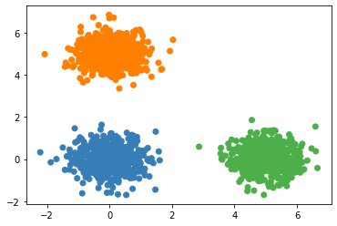
colors = np.array(['#377eb8', '#ff7f00', '#4daf4a', '#a65628'])
plt.scatter(X[:, 0], X[:, 1], color = colors[clusters]

2.2.4 k-means in sklearn

import numpy as np
import matplotlib.pyplot as plt
from sklearn.cluster import KMeans

k = 3
random_state = 6
y_pred = KMeans(n_clusters=k, random_state=random_state).fit_predict(X)

colors = np.array(['#377eb8', '#ff7f00', '#4daf4a', '#a65628'])
plt.scatter(X[:, 0], X[:, 1], color = colors[y_pred])

Compare The running time of my code is at most half of that of KMeans in sklearn. There is still much space to improve since I still use for loop and did not use Broadcast very well.

2.3 Cons

(1) Need the number of clusters $k$ first.

(2) Sensitive to the initial centroids. For example, the unsuitable initial centroids make the result looked awful (K-means++ Algorithm could help to avoid that)

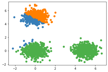
(3) Suitable for only circle like distribution, and therefore does not work well on other distribution shapes (use Spectral Clustering instead). For example: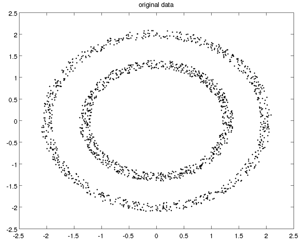

(4) Sensitive to noise. (Could use the median but not mean to generate centroids) (K-medoids Algorithm could help to avoid that)

3. Spectral Clustering

Links Back Unsupervised Learning - Dimensionality Reduction - Isomap

3.1 Intro

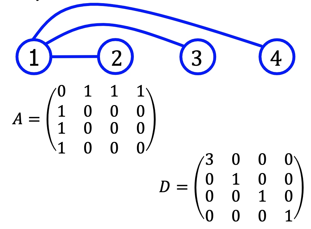
First, let’s make some definitions Adjacency Matrix: $A\in R^{m\times m}$

Degree Matrix: $D\in R^{m\times m}$

Laplacian Matrix:

examples:

• Graph A

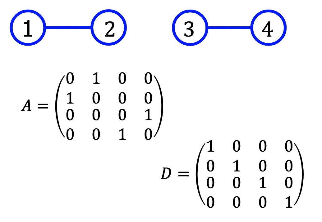
• Graph B

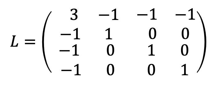
3.2 Laplacian Matrix

\(L=D-A\)

拉普拉斯矩阵是我们主要的关注对象，它有很多很有用的性质，其中最重要的为:

The multiplicity of the eigenvalue 0 corresponds to the number of connected components (0特征值的重数等于不相连团的个数)

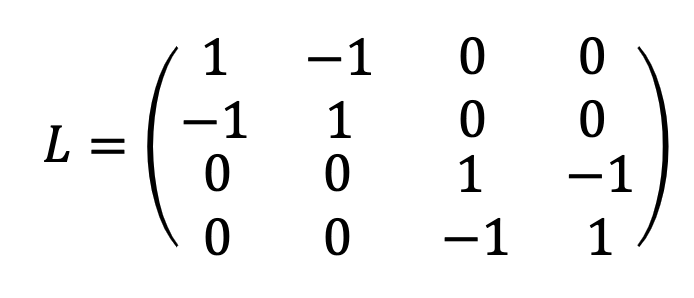
For example, the following graph containin 2 connected components has 2 eigenvectors with zero eigenvalue: $[1,1,0,0]^T$ and $[0,0,1,1]^T$

Moreover, if the graph has $k$ clusters with the following $L$:

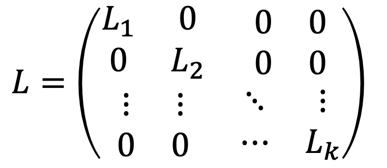
then there will be more $k$ eigenvectors with zero egivenvalue

3.3 Spectral Clustering

谱聚类本质上就是对于拉普拉斯矩阵的特征根进行聚类，首先给出常规流程

(1) Given $m$ data points, threshold $\epsilon$

• construct adjacency matrix \(A^{ij}=\begin{cases} 1 &\text{if }\|x^i-x^j\|^2\leq\epsilon\\ 0 &\text{else} \end{cases}\)

• construct degree matrix \(D^{ij}=\begin{cases} \sum_{k=1}^mA^{ik} &\text{if }i=j\\ 0 &\text{if }i\ne j \end{cases}\)

• then Laplacian matrix $L=D-A$

(2) Compute $k$ eigenvectors $v^1,…,v^k$ of $L$, corrosbonding to $k$ smallest eigenvalues

(3) Run K-means on $Z=[v^1\text{ }…\text{ }v^k]$ by treating each row as a new data point

3.4 An Extreme Example

考虑如下情况

we have $m=4$, let $k=2$, then 2 eigenvectors with smallest eigenvalues (actually equal to zero) are $[1,1,0,0]^T$ and $[0,0,1,1]^T$. Then construct $Z$: \(Z=\begin{bmatrix} 1 & 0\\ 1 & 0\\ 0 & 1\\ 0 & 1\\ \end{bmatrix}\)

很显然，此时如果对 $Z$ 做 K-means, 前两点会被归为一类，后两点另一类

Based on the above example, for more general cases 有可能整张图是一个 connected components, 但是有很多地方都是藕断丝连的。此时只有一个 eigenvector 对应的特征值为零，因此为了分出 $k$ clusters，就还需要再找出 $k-1$ 个 eigenvectors 对应尽可能小的特征值（每个特征根都表示了一个 cluster）