1. EOQ Model

Notations & Assumptions: $t = 1$ means one year.

• $D=D(1)$ yearly demand (deterministic and constant)
• $q$ decision variable (order size)
• $p$ unit cost
• $K$ set up cost per order
• $h$ is holding cost per unit per time
• $L=$ lead time (下订单后运到仓库所需时间)
• no backorder, no shortage

What is backorder? A backorder is an order for a good or service that cannot be filled at the current time due to a lack of available supply. The item may not be held in the company’s available inventory but could still be in production or in transition

1.1 General Case (Lead Time = 0)

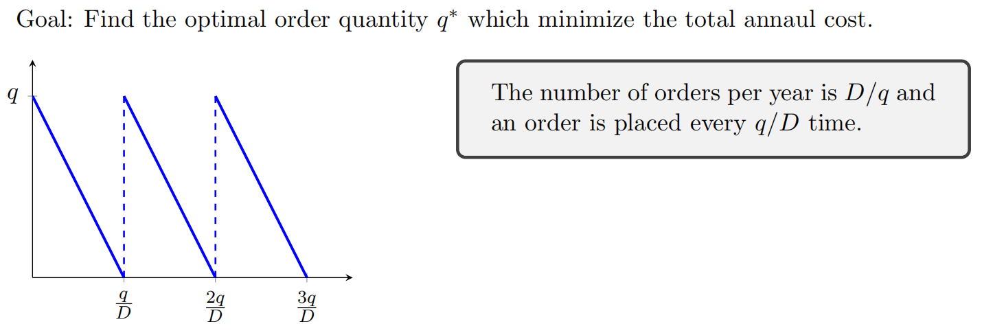
EOQ(Economic Order Quantity) \(\boxed{q^*=\sqrt{\frac{2KD}{h}}}\)

How we get that?

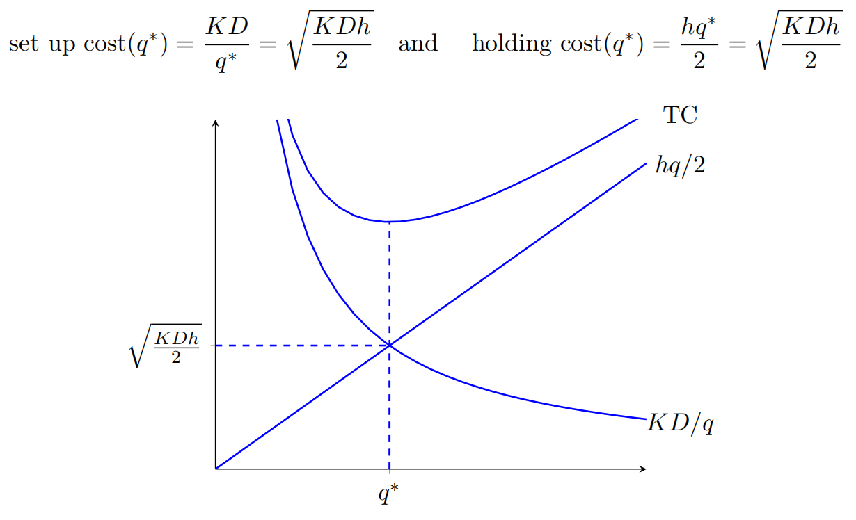
• Let $TC$ represent the annual total cost. Note that this total cost depends on $q$, thus： \(\begin{aligned} TC(q) &= \text{setup cost+annual purchasing cost+annual holding cost}\\ &= K\frac{D}{q} + pD + h\frac{q}{2} \end{aligned}\)

• Then we could get EOQ by solving: \(\frac{d}{dq}TC(q)=-\frac{KD}{q^2}+\frac{h}{2}=0\)

• Why EOQ is a minimization solution? second derivative > 0

Some interesting facts:

1. Even the equation of $q^$ is not related to $p$, while $p$ will often affect $h$ and then affect $q^$
2. The optimal $q$ is achieved when the setup cost and holding cost are equal 这是由 $TC(q)$ 的公式决定的，如果再加一项关于 $q$ 的公式就不会这么巧了

1.2 Lead Time > 0

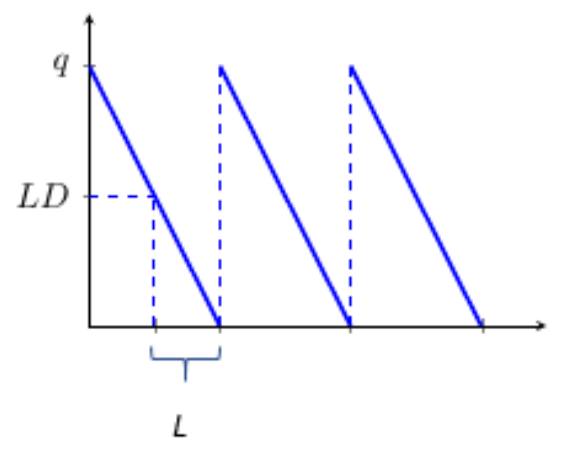
When $L > 0$ and is a constant, we should place an order when the stock level is large enough to cover the demand during the lead time which is $LD$. Thus the reorder point $r$ is $r = LD$

• If $LD<EOQ$, $r=LD$
• If $LD>EOQ$, $r=LD\text{ mod }EOQ$

For a long lead time, the pipline cost(or trasit cost) is sometimes considered and is equal to $q(Lh)(D/q) = DLh$

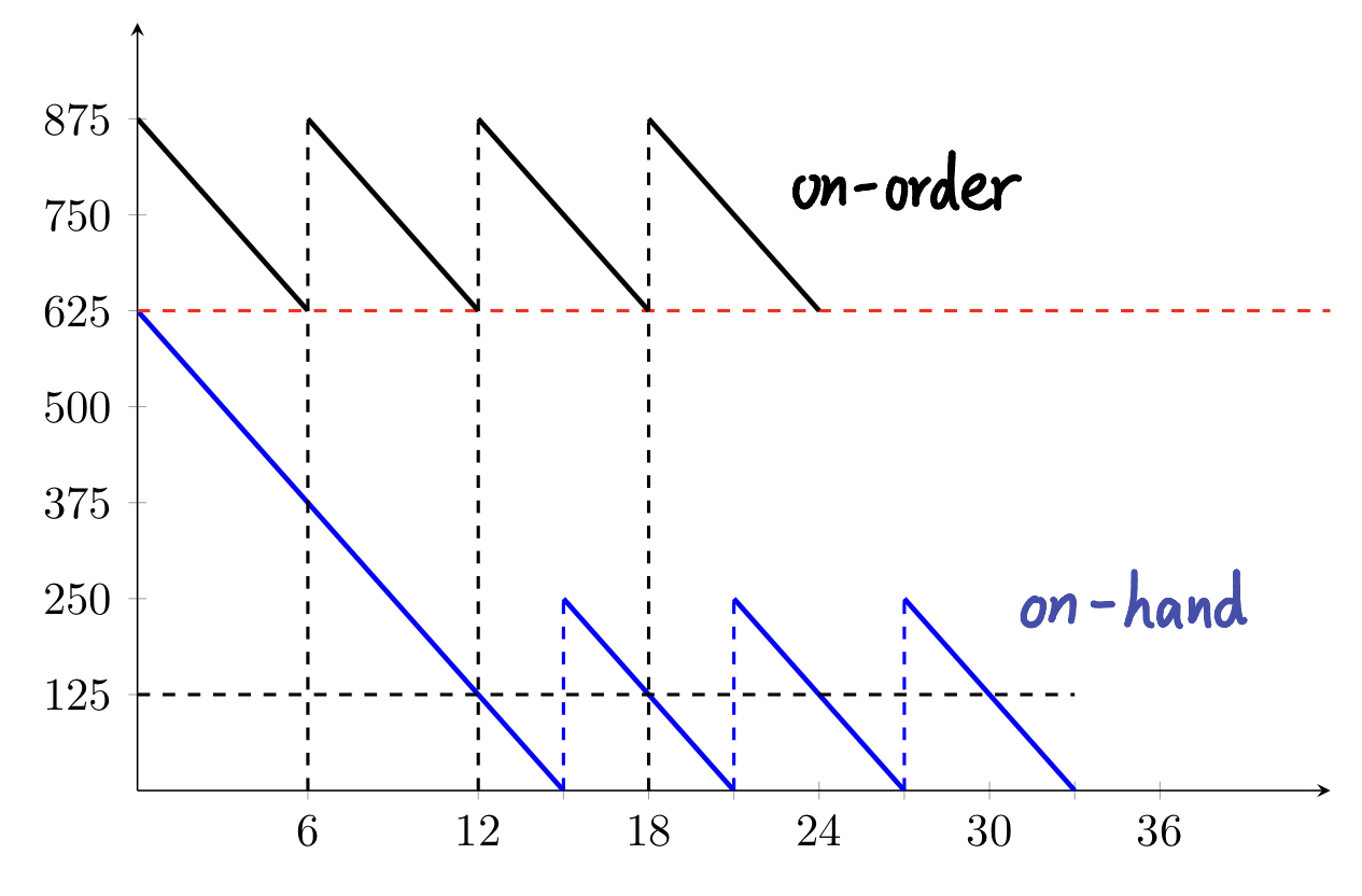
How do we simulate an inventory policy with $LD>q$? Keep on-order inventory and place an order whenever the on-order inventory is equal to $r$ \(\text{on-order = on-hand + backordered(negative) + in-transit}\)

For example, when $q=250,r=625$, when start at on-hand inventory at $OHI=625$, we need to immediately order a $q$. Therefore our on-order inventory at start will be $q+r=875$

1.3 What if …?

What if $D$ is not a constant but a random variable? EOQ is recommended when

1. squared coefficient of variantion (SCV) $=Var(D)/E^2[D]<0.2$
2. OR standard diviation (std) $<0.45E[D]$

2. Gaussian Demand Process

Definitions: Let $D(t)$ represent the demand during time $t$ (in years) and $E[D(1)]=\bar{d}, Var[D(1)]=\sigma_d^2$. Then a Gaussian demand process has \(D(t)\sim N(t\bar{d},t\sigma_d^2)\)

反过来，如果说上述公式是从大时间的分布(1年)来得出小时间的分布，我们还可以用 CLT 来从小时间的分布得出大时间的分布:

1. $n>30$, e.g. week to year use CLT weekly demand $X_i$ are idd with $\mu,\sigma^2$ $D=\sum_{i=1}^{52}X_i\sim N(52\mu,52\sigma^2)$
2. $n<12$, e.g. month to year cannot use CLT but if monthly demand $X_i$ are idd and gaussian with $\mu,\sigma^2$ $D=\sum_{i=1}^{12}X_i\sim N(12\mu,12\sigma^2)$