# Optimizing Factory Performance

1. Introduction

2. History and Implications

Three primary enemies of factory (or supply chain or organizational):

Complexity
Variability
Lackluster leadership

3. Terminology, Notation, and Definitions

3.1 Factory: Definition and Purpose

A factory is a processing network through which jobs and information flow and within which events take place.

From a more scientific perspective, an alternate and more revealing definition of a factory may be developed, specifically:

A factory is a nonlinear, dynamic, stochastic system with feedback.

Job Process

Job process steps (a.k.a. operations) include

Assembly or transformation: an activity resulting in or directly supporting a physical and measurable change to the job
Transit of the job from one machine to the next
Inspection of the job

Workstation events

Concurrent with the flow of jobs through a factory are events that occur within the factory’s workstations. These events serve to reduce the availability of the machines that form the workstation and, subsequently, the overall availability of the workstation itself. The degradation imposed by such events on the workstation—and the factory—in turn, will have an impact on factory performance. (例如机器的维护和检查)

Workstation events are:

Maintenance of a machine
Repair of a machine
Inspection of a machine
Qualification of a machine
Setup of a machine

For example, a maintenance event may occur according to a schedule (e.g., perform a maintenance event every week), or according to usage (e.g., perform a maintenance event on the completion of every 500 jobs)

3.2 Factory Process-Flow Models

Every factory (or supply chain or business process) supports a process flow. There are several ways to represent this flow, for example:

Workstation-centric model: a workstation consists of one or more machines that support identical or nearly identical processing functions
Process-step-centric model: an operation conducted within a workstation (and, quite possibly, by means of the support of only a subset of the machines in the workstation) or is a transit step between workstations.

Model 1: Workstation-centric Model and Reentrancy

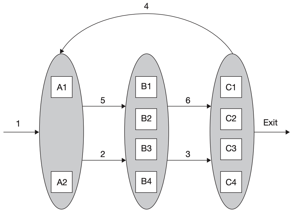
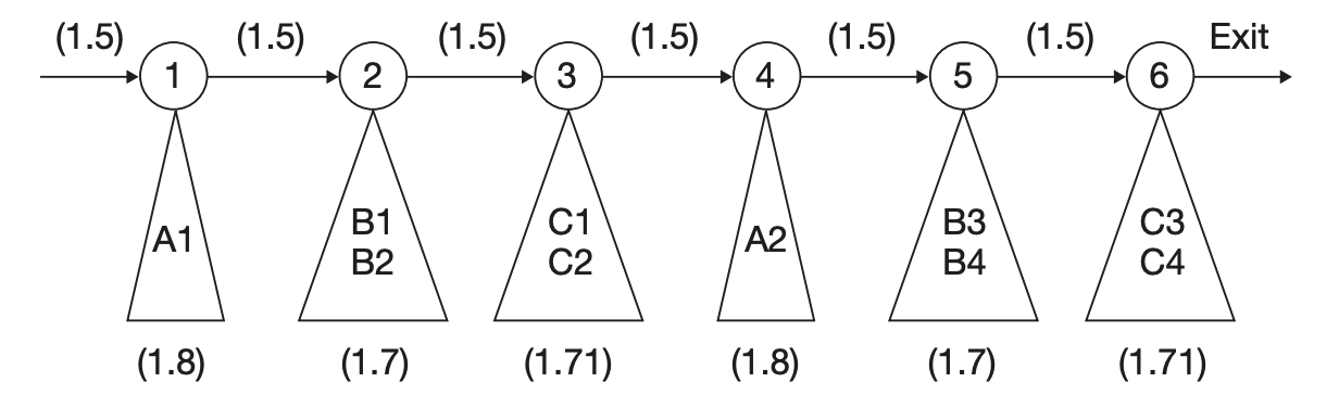
The following picture depicts a simple factory consisting of:

3 work stations (A, B, and C) (包括 transit operations)
7 machines (A1, A2, …)
5 operations (arrows 1, 2, …) (这里的箭头表示的不是 intralogistics)

Figure 3.1

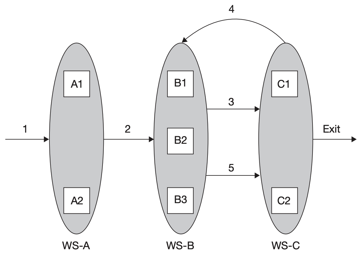
Def: Degree of Reentrancy (DoR) $DoR = \frac{\# operations}{\# work stations} = \frac{5}{3}$

DoR differs a lot for different types of factory:

automobile assembly lines have little, if any, reentrancy (the ideal assembly line has none)
semiconductor wafer fabrication facilities, or “fabs”, typically have factory DoR values ranging from 3 to 5 or even more—with individual nests that may have DoRs in the double digits.

We next consider two other, more traditional (in that they do not include reentrancy) workstation-centric models:

(1) Flowshop factory

Figure 3.2

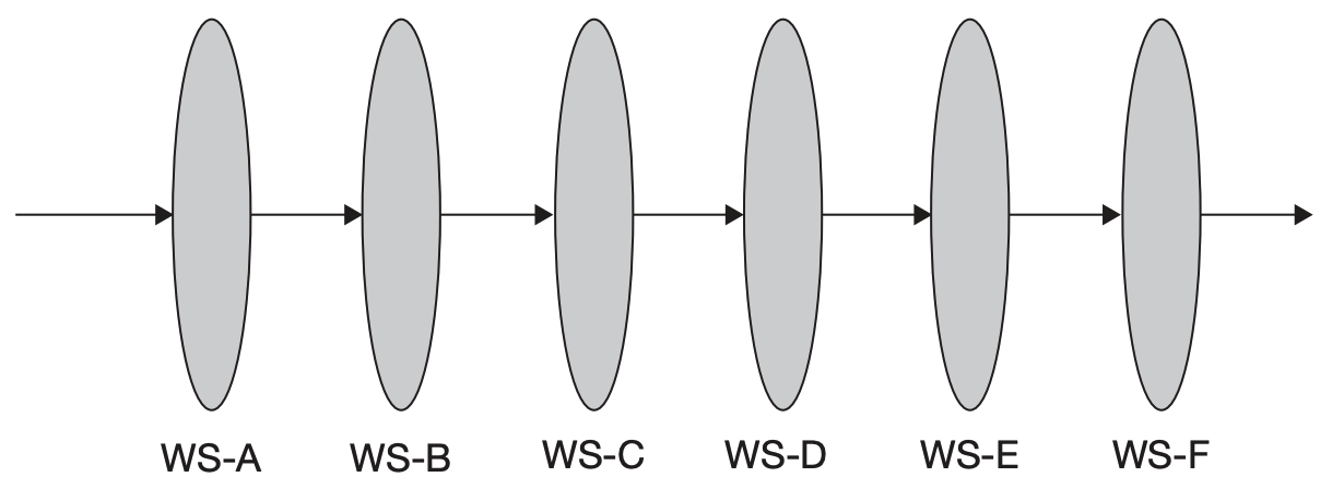
Each job follows precisely the same pathway
Each workstation supports just one process step
No passing of jobs: if two jobs enter the factory in, say, the job sequence J1 and J2 they must enter and leave each workstation in that same sequence

(2) Jobshop factory

Figure 3.3

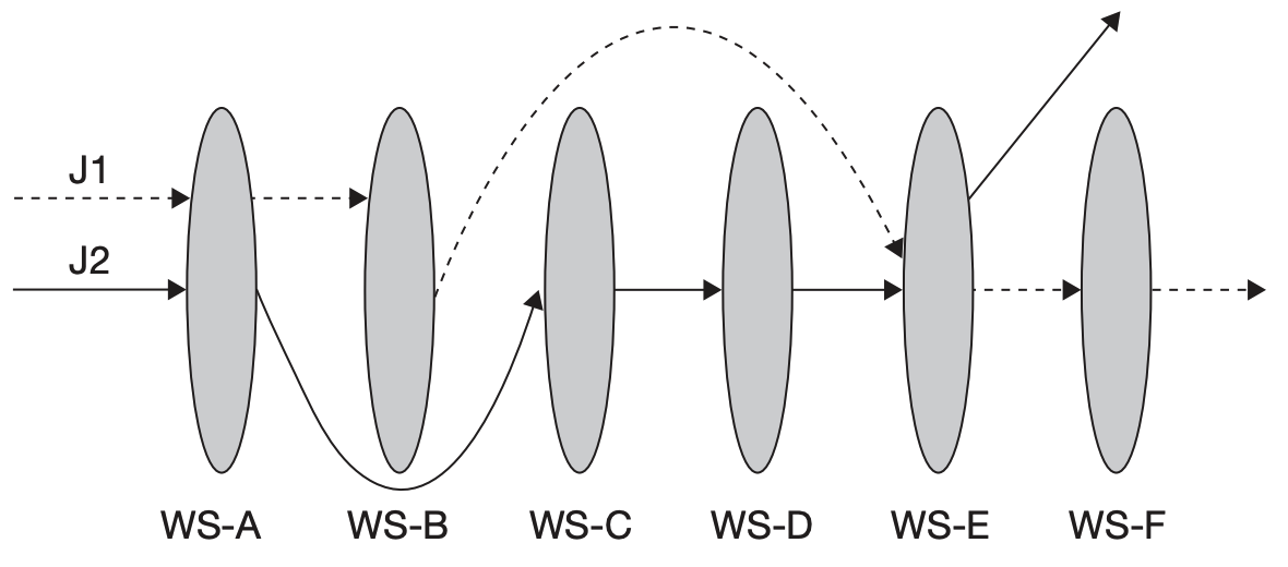
Each job that enters the factory may follow a different process flow path (J1 vs. J2)

Model 2: Process-step-centric Model

According to Figure 3.1, if we know which machines are capable of supporting (e.g., qualified to conduct or be assigned to) each process step, we can convert that workstation-centric model into a process-step-centric model:

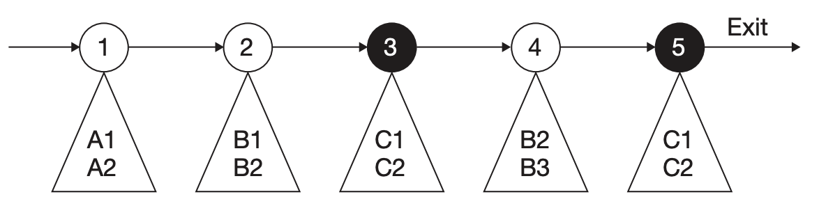
Why this model is also important:

it indicates not only the process step flow but also the precise support responsibilities of each machine in the factory.

3.3 Factory Definitions and Terminology

Factory Types

Flowshops vs. Jobshops (as mentioned just above)
Factories with (i.e., DoR > 1) and without reentrancy (i.e., DoR = 1)
Synchronous factories: every job flows through the factory at the same constant speed, such as bottles in a beverage bottling plant
Asynchronous factories: each job, as in semi-conductor fabrication, may flow through the factory at different speeds and in addition may remain temporarily held in a queue
High-mix factories (e.g., those that process numerous job types)
Low-mix factories (e.g., those that process only a limited number of job types)
Low-volume factories (e.g., those that process only a relatively limited number of jobs per time period, such as aircraft manufacturers or research and development factories that produce only prototypes of a product)
High-volume factories (e.g., those that process a large number of jobs per time period, such as high-volume semiconductor wafer fabrication facilities)
Combinations: (1) High-mix, low-volume factories (2) High-mix, high-volume factories (3) Low-mix, low-volume factories (4) Low-mix, high-volume factories
Factories involving various combinations of the preceding features

3.4 Jobs and Events

Job Types

Jobs may require either assembly, transformation, the combination. Furthermore, a job may flow through the factory as a single unit (e.g., as an automobile), as a lot (e.g., as a “container” consisting of a number of silicon wafers), or as a batch (e.g., a group of either individual jobs or lots).

Two primary types of batches:

parallel batch: batch 中的 jobs 会被同时处理 (same process time). Batch 的目的在于 reduce setup time (each batch undergoes just one setup in front of the batching machine). 例如, 陶瓷烧制机器允许同时烧制多个陶瓷坯
series batching or cascading: batch 中的 jobs 会被顺序处理. 同样能够 reduce setup time because each cascade undergoes just one setup prior to entry into the cascading machine or workstation.

Job States

Value-added processing: an actual assembly or transformation operation

Non-value-added processing:

Rework
Transit
Inspection/test
Waiting, including
- Waiting as an individual job for processing at a nonbatching/noncascading process step
- Waiting for a batch (or cascade) to form in front of a batching/cascading process step
- Waiting in a batch (or cascade) as part of the queue formed in front of a batching/cascading process step
- Waiting in a “set aside” state (e.g., the job is removed temporarily from the production line)

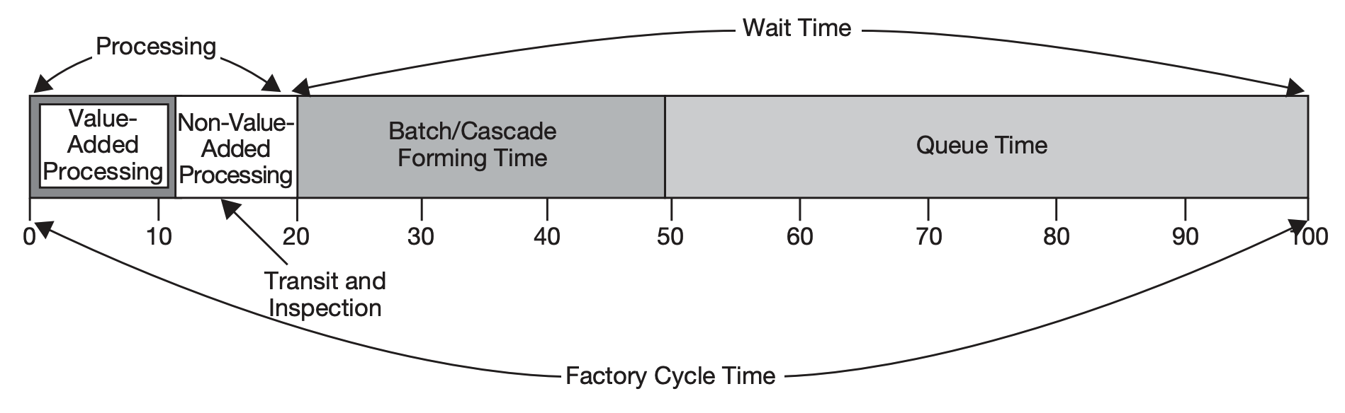
如图所示, 在很多真实工厂中, non-value-added processing 的时间占了相当大的一部分

Event Types

Events are activities that are conducted within a workstation rather than on a job

Preemptive Events: occurs during the processing of a given job (or batch). The processing of the job must stop and cannot proceed until recovery from the preemptive event:

Unscheduled downs
Power outages or voltage/current spikes
Unanticipated supply outages and replenishment

Nonpreemptive Events: occurs (or can be scheduled to occur) during a period in which the machine is not processing a job:

Scheduled maintenance
Unscheduled downs (i.e., those that happen to not occur during processing)
Inspections and engineering tests
Qualifications
Setups
Scheduled operator breaks (e.g., biobreaks or meetings)

3.5 Workstations, Machines, and Process Steps

Workstations

A given workstation consists of one or more machines, each dedicated to an identical or nearly identical processing function.

Machine States

Processing: busy in support of job processing (i.e. those involving assembly or transformation, rework, transit, and inspection/test of a job)
Blocked: machine is up and running, 但是正在进行一项和 the support of an actual process step 无关的进程, 例如:
- those involving inspection/ test of the machine
- those involving qualification
- those involving setup
- those on hold waiting for the arrival of priority job
Idle: machine is up, running, and qualified but there are no jobs either in the machine or waiting for the machine
Down: machine is down due to either a sheduled or unscheduled event

Process Steps

The key attributes of capacity and cycle time are determined by the support provided to each individual process step rather than each functional area.

{CT}_{f} = \sum_{p s = 1}^{P} {CT}_{p s}

${CT}_{f}$ : cycle time of the entire factory
${CT}_{p s}$ : cycle time of process step $p s$
$P$ : total number of process steps in the factory

The capacity of a factory is determined by the bottleneck (i.e., constraint or choke point) process step, not necessarily a bottleneck workstation

3.6 Performance Measures

Notation

Define the performance measure for an entity as the following format:

{Measure}_{entity} (specific entiry designation)

For example:

${CT}_{p s} (9)$ cycle time of process step number 9
${PR}_{m} (B 3)$ process rate of machine 3 in workstation B (B3)

entity

\begin{aligned} p s & = process step, where p s = 1, . . ., P \\ m & = machines, where m = 1, . . ., M \\ w s & = workstations, where w s = 1, . . ., W \\ f & = factory \end{aligned}

Process-Step Performance

${TH}_{p s}$ (jobs/ time): Process-step average throughput rate
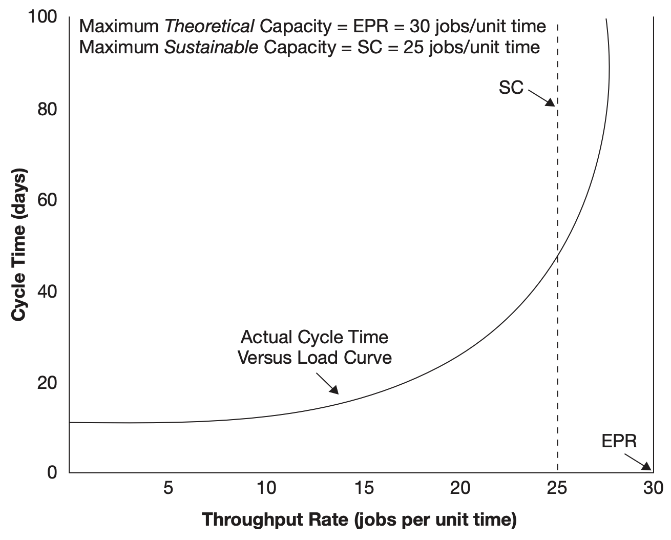
${EPR}_{p s}$ (jobs/ time): Effective process rate or maximum theoretical capacity the capacity of the machines supporting that step in the absence of any variability. (upper bound of the process-step capacity)
${SC}_{p s}$ (jobs/ time): Process-step maximum sustainable (可持续的) capacity
${CT}_{p s}$ : Process-step cycle time the elapsed time between the arrival of the job at the queue (if one exists) in front of the process step and its departure on completion of the operation
${AR}_{p s}$ (jobs/ time): Arrival rate at the process step
${DR}_{p s}$ : Departure rate from the process step

Figure: $SC$ (max sustainable capacity) vs. $EPR$ (max theoretical capacity)

Machine Performance

${TH}_{m}$
${EPR}_{m}$
${SC}_{m}$
$A_{m}$ : Availability
${PR}_{m}$ : Raw process rate
$B_{m}$ : Busy time rate
${DT}_{m}$ (time per time): Machine downtime rate
$ρ_{m}$ : Machine occupancy rate (utilization)
${PCC}_{m}$ : Machine production control channel width
${MTBE}_{m}$ : Mean time between machine down events (但这期间 machine 不一定在运行)
${MTTR}_{m}$ : Mean time to recover from machine down events

Machine Availability the percenrage of the time the machine is up, running, and qualified to process jobs. = 可用时间 / (可用时间 + 维修时间), 注意这里的可用时间不等于工作时间 (busy time)

A_{m} = \frac{{MTBE}_{m}}{{MTBE}_{m} + {MTTR}_{m}}

Machine Raw Process Rate 理想状态下机器的最大产能 (maximum number of jobs/ time)

Using ${PT}_{m}$ to denote a machine’s raw process time,

{PT}_{m} = \frac{1}{{PR}_{m}}

Machine Effective Process Rate: machine maximum theoretical capacity (不考虑 variability)

{EPR}_{m} = A_{m} \times {PR}_{m}

Using ${EPT}_{m}$ to denote a machine’s effective process time,

{EPT}_{m} = \frac{1}{{EPR}_{m}}

Machine Busy Rate: the percent of time, over a given time period, spent in the busy state

B_{m} = \frac{{AR}_{m}}{{PR}_{m}} = {AR}_{m} \times {PT}_{m}

${AR}_{m} =$ Arrival rate at the machine
${PR}_{m} =$ Raw process rate of the machine
${PT}_{m} =$ Raw process time of the machine

Machine Occupancy Rate (Utilization): percentage of the available time in the busy state

ρ_{m} = \frac{B_{m}}{A_{m}}

ρ_{m} = \frac{{AR}_{m}}{{EPR}_{m}}

Machine Production Control Channel

{PCC}_{m} = \frac{A_{m} - B_{m}}{A_{m}} = 1 - ρ_{m}

Workstation Performance

A discussion of the performance measures of a workstation will make sense in general only if the workstation supports a single process step and every machine in the workstation is qualified to support that process step and only that process step. (对于不符合这种假设的其他 workstation, 会在之后的章节讨论到)

\begin{aligned} {TH}_{w s} & = \sum_{m = 1}^{M} {TH}_{m} & throughput rate \\ {EPR}_{w s} & = \sum_{m = 1}^{M} {EPR}_{m} & theoretical capacity \\ A_{w s} & = \sum_{m = 1}^{M} A_{m} / M & availability \\ B_{w s} & = \frac{{AR}_{w s}}{{PR}_{w s}} & busy time rate \\ ρ_{w s} & = \frac{B_{w s}}{A_{w s}} = \frac{{AR}_{w s}}{{EPR}_{w s}} & occupancy rate \\ {PCC}_{w s} & = 1 - ρ_{w s} \end{aligned}

需要注意的是: $\text{SC}{ws} $s u s t a i n a b l e c a p a c i t y, 和$ \text{SC}{m}$ 没有求和相等的关系, 而是受到多种其他情况的影响

Factory Performance

${CT}_{f}$ : Factory cycle time
${CTE}_{f}$ : Factory cycle-time efficiency
${TH}_{f}$ : Factory throughput rate (rate of flow of jobs through the entire factory)
${SC}_{f}$ : Factory maximum sustainable capacity, determined by the maximum factory cycle time that the firm can tolerate
${EPR}_{f}$ : Factory maximum theoretical capacity
Product lead time
Factory moves
${WIP}_{f}$ : Factory inventory

Factory Cycle Time

{CT}_{f} = \sum_{p s = 1}^{P} {CT}_{p s}

Factory Cycle-Time Efficiency

{CTE}_{f} = \frac{{Process Time}_{f}}{{CT}_{f}}

Factory Inventory: Little’s Law

{WIP}_{f} = {TH}_{f} \times {CT}_{f}

3.7 Put It All Together

A simple but meaningful example. 这个例子不仅展示了工厂内部各种性能指标的计算和相互关系, 更重要是, 它强调了降低 dor

3.7.1 Workstation-Centric Model (Initial)

Let’s consider a factory with:

arrival rate ${AR}_{f} = 1.5$ jobs/ hr
operates $168$ hrs/ week
degree of reentrancy $DoR = 2$
no variability

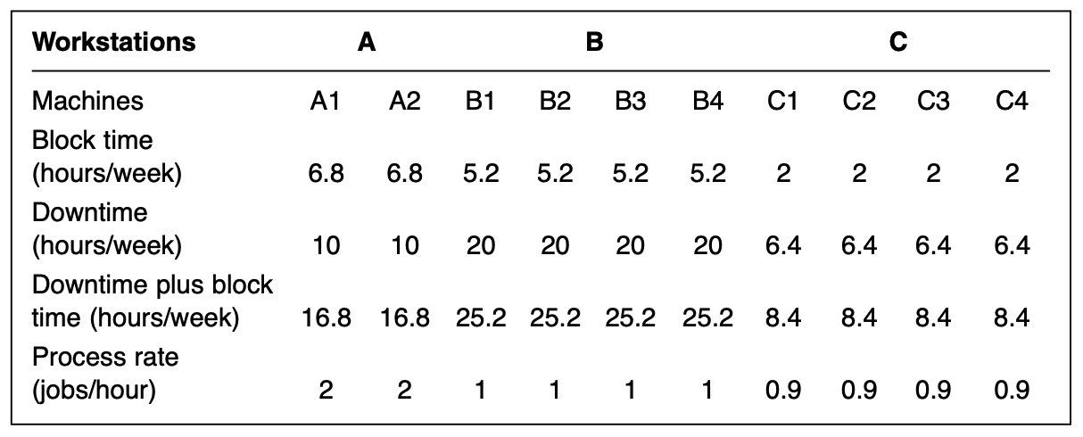
Using the above data, we may compute the effective process rate ${EPR}_{m}$ of each machine:

A_{m} = \frac{T - ({DT}_{m} + {BT}_{m})}{T}

{EPR}_{m} = A_{m} \times {PR}_{m}

For example, for machine $A1$ :

$A_{m} (A1) = (168 - 16.8) / 168 = 0.9$
${EPR}_{m} (A1) = 0.9 \times 2 = 1.80$ jobs/ hr

Then after calulating for each machine, we can update the table above as follows:

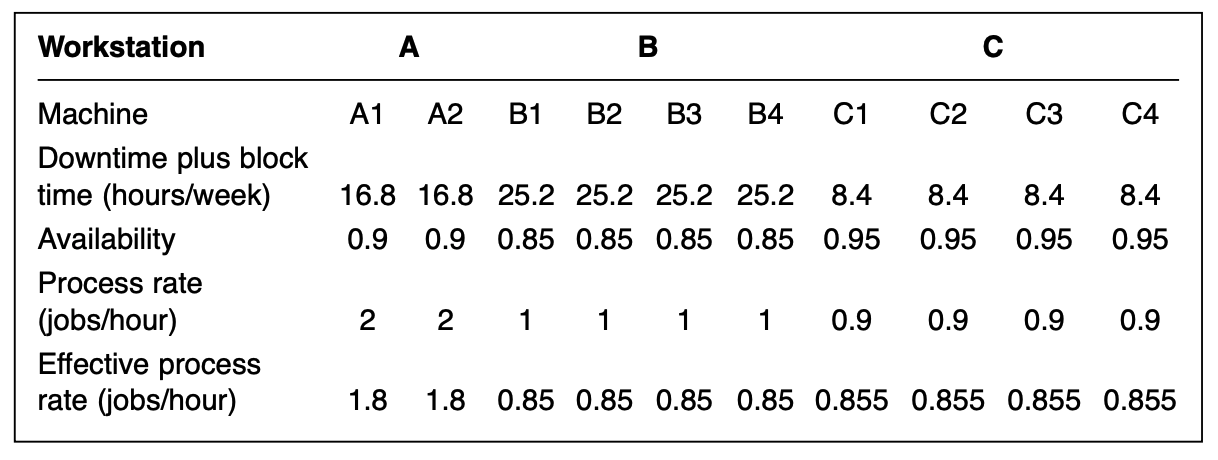
The throughput rate imposed on each workstation is $1.5 + 1.5 = 3$ jobs/ hr. And the maximum theoretical of each workstation can be calculated using the table above:

${EPR}_{w s} (A) = 2 \times 1.8 = 3.6$ jobs/ hr
${EPR}_{w s} (B) = 4 \times 0.85 = 3.4$ jobs/ hr
${EPR}_{w s} (C) = 4 \times 0.855 = 3.42$ jobs/ hr

All these ${EPR}_{w s}$ is larger than $3$ , which seems to show that each workstation is capable of supporting the job flow.

3.7.2 Proccess-Step-Centric Model

We have to firstly allocate machines to process steps in each workstation, for example:

Process step 1 $\to$ machine A1
Process step 2 $\to$ machines B1 and B2
Process step 3 $\to$ machines C1 and C2
Process step 4 $\to$ machine A2
Process step 5 $\to$ machines B3 and B4
Process step 6 $\to$ machines C3 and C

Using the above allocated process-step-centric model, a new fully decoupled workstation-centric model can be constructed.

3.7.3 Workstation-Centric Model (Decoupled)

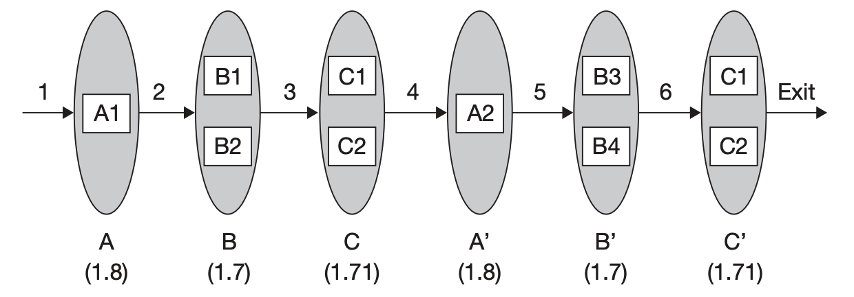
小括号里的数据表示新的的 workstation 的 ${EPR}_{w s}$ (基于 Section 3.7.1 的第二张 machine 表计算)

Then we can calculate the workstation occupancy rate, and find the bottleneck is workstation $B$ and $B^{'}$ , or process steps $2$ and $5$

ρ_{w s} = \frac{{TH}_{w s}}{{EPR}_{w s}}

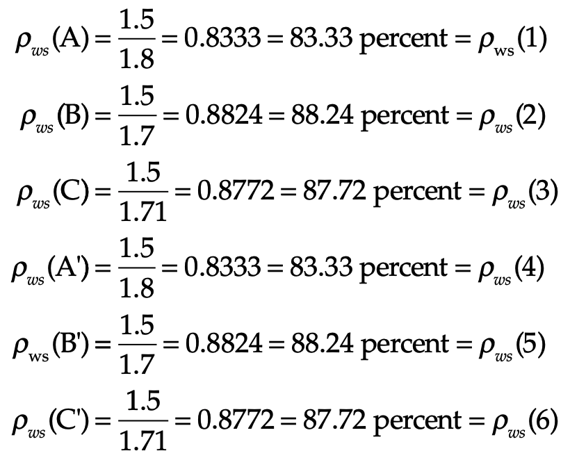
Finally, let’s determine the cycle time of the factory. Assuming:

no varaiablity in machines, procee rates, and throughput rates
the time required to move from one nontransit process step to another is 5 minutes

(以下公式中的 ${EPR}_{p s}$ 来自于本 Section (3.7.3) 第一张图中 workstation 下方的小括号)

{CT}_{f} = 6 \times \frac{5}{60} + \sum_{p = 1}^{6} {CT}_{p s} (p) = 0.5 + \sum_{p = 1}^{6} \frac{1}{{EPR}_{p s} (p)} = 3.5972 hrs

{WIP}_{f} = {TH}_{f} \times {CT}_{f} = 1.5 \times 3.5972 = 5.9358 jobs

在这个例子中, 我们通过从 initial workstatio-centric model 到 decoupled workstation-centric model 的转变, 把 $DoR$ 降低到了 $1$ 。尽管对于绝大多数 real factories, 我们无法实现降低 $DoR$ 到 $= 1$ 这样的转变, 但是我们仍可以通过尽可能的减小 $DoR$ 来简化问题

同时也要注意, 这里最后的 cycle time 是及其理想的, 因为我们假设一个 product 可以被一个 workstation 中的多台 machines 同时处理, 遑论我们还没有考虑 variablity 的巨大影响

代码示例: A Simple Cylce Time Simulation FabSim_1_3.py

4. Running a Factory: In Two Dimensions

http://nbpfabtime01/FabTime717/ChartPage.html? starttime=2022-8-31%205%3A30%3A0& endtime=2023-9-1%205%3A30%3A0& toolslike=N_ACID16& basicstateslike=Unsch& timeumid=4& chartsortfield1=Tool& chartsortfield2=TranTime& stripecolor=Black& stripeaxis=Y& width=644& height=400& grid=None& datavalues=None& horizontal=0& pagemode=2& activemode=Javascript& chart=TOOLSTATETRANLIST& chartview=0& tableview=0& factoryid=1& goaluserid=951& editchart=0& uid=2023123128551694028416

5. Variability

5.1 Measuring Variability

$C o V = σ / μ$ : coefficient of variation

$C_{A R}$ : cov of Arrivals (interarrival times)

In general, $C_{A R}$ of batch arrivals is larger than that of continuous arrivals (因为 batch 内部的 interarrival time = 0, 这会导致 $μ$ 变得很小, 因此 cov 变得很大)

$C_{P T}$ : cov of Raw Process Times

$C_{P T} (p s)$ : … of a given process step

#### CoV of Effective Process Times

For a nonreentrant ( $DoR = 1$ ) workstation:

C_{E P T}^{2} (p s) = C_{0}^{2} + A (1 - A) \frac{M T T R}{P T} + C_{D E}^{2} A (1 - A) \frac{M T T R}{P T}

$C_{0}$ : inherent variability of the process times of the machines
$C_{D E}$ : cov of blocked and down events
$A$ : average availability of the machines
$M T T R$ : mean time to recover from blocked and down events
$P T$ : average raw process time of the machines (理想情况下, 完成一次 process 所需要的时间)

Example: For process step 7, we know

mean time between down events $M T B E = 90$ , $M T T R = 10$
$C_{0} = C_{P T} (7) = 0.042$ (approximated), $C_{D E} (7) = 1.5$
$P T (7) = 1$ hour

Then $A = 90 / (90 + 10) = 0.9$ , and finally:

C_{E P T}^{2} (7) = {0.042}^{2} + 0.9 (1 - 0.9) \frac{10}{1} + {1.5}^{2} \times 0.9 (1 - 0.9) \frac{10}{1} = 2.93

可以看到即使 the inherent variability of the process times of the machines ( $C_{0}$ ) 很小, 但是由于 blocked and down events 及其 cov 很大 ( $M T T R$ , $C_{D E}$ ), 因而使得 effective process times 的 cov 变得很大

不难发现, assume no blocked events, 如果我们能够 divide scheduled down events into more frequent, smaller segments, 那么在不改变 availability ( $A$ ) 的情况下, 就能够通过减小 $M T T R / P T$ 来显著降低 cov of effective process times

5.2 Three Fundamental Equations

Equation 1: Little’s Law

W I P = C T \times T H

Equation 2: Pollaczek Khintchine

P-K equation is used to predict the cycle time of a factory, a portion of a factory, or some individual workstation. However, here, we will focus on the cycle time at the process-step level

Factors covered:

$C T_{p s}$ : cycle time of the process step
$C_{A R}$ : cov of arrivals at the process step (time between interarrivals)
$C_{E P T}$ : cov of effective process times of the machines that support the process step
$E P R_{p s}$ : effective process rate (maximum theoretical capacity) of each of the **identical machines** that… (如果 that process-step is supported by a single machine, then $E P R_{p s} = E P R_{m}$ )
$A$ : average availability of the machines that…
$ρ = T H / E P R$ : average occupancy (a.k.a. utliization) of the machines that… (要注意辨别这里的 $T H$ 和 $E P R$ , 例如对于理想工厂 with no reentrancy, 每个 workstation 串联在一起, 任意 workstation 内的 machines 完全相同且都能独立完成一个 process-step, 那么此时 $ρ = T H_{f} / E P R_{w s} = T H_{f} / (m \times E P R_{m})$ )
$B S$ : batch size of the machines that…
$A R$ : arrival rate of the jobs arriving at the process step
$m$ : number of (identical) machines supporting the process step.

To determine the cycle time of a process step supported by $m$ **nonreentrant and nonbatching** machines.

C T_{p s} = \underset{wait in queue time}{\underset{⏟}{(\frac{C_{A R}^{2} + C_{E P T}^{2}}{2}) [\frac{ρ^{\sqrt{2 (m + 1)} - 1}}{m (1 - ρ)}] (\frac{1}{E P R_{p s}})}} + \underset{effective process time}{\underset{⏟}{\frac{1}{E P R_{p s}}}}

rho = TH_f/EPR_ws

CT_queue = ((cov_AR**2+cov_EPT**2)/2) * (rho**(np.sqrt(2*(m+1))-1) / m / (1-rho)) * (1/EPR_m)
CT_processing = 1/EPR_m
CT_ws = CT_processing + CT_queue

so for a single machine ( $m = 1$ ):

C T_{p s} = \underset{wait in queue time}{\underset{⏟}{(\frac{C_{A R}^{2} + C_{E P T}^{2}}{2}) [\frac{ρ}{(1 - ρ)}] (\frac{1}{E P R_{p s}})}} + \underset{effective process time}{\underset{⏟}{\frac{1}{E P R_{p s}}}}

For the process step supported by $m$ machines empolying batching:

C T_{p s} = \underset{batch forming time}{\underset{⏟}{\frac{B S - 1}{2 A R}}} + \underset{wait in queue time}{\underset{⏟}{(\frac{C_{A R}^{2} / B S + C_{E P T}^{2}}{2}) [\frac{ρ^{\sqrt{2 (m + 1)} - 1}}{m (1 - ρ)}] (\frac{1}{E P R_{p s}})}} + \underset{effective process time}{\underset{⏟}{\frac{1}{E P R_{p s}}}}

Equation 3: Linking (Propagation of Variability)

employed to estimate the cov of the jobs departing a given process step.

Given $m$ machines and no reentrancy:

C_{D R}^{2} = 1 + (1 - ρ^{2}) (C_{A R}^{2} - 1) + (\frac{ρ^{2}}{\sqrt{m}}) (C_{E P T}^{2} - 1)

rho = TH_f / EPR_ws
cov_DR = np.sqrt(1 + (1-rho**2)*(cov_AR**2-1) + (rho**2/np.sqrt(m))*(cov_EPT**2-1))

so for a single machine ( $m = 1$ ):

C_{D R}^{2} = ρ^{2} \times C_{E P T}^{2} + (1 - ρ^{2}) \times C_{A R}^{2}

Propagation:

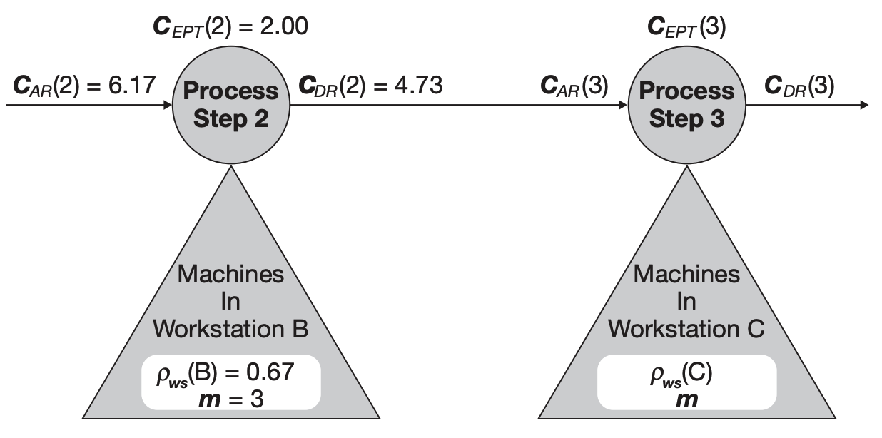
如上图, assume all machines in the workstation B support process step 2 and only that process step, 已知 $C_{A R} (2), C_{E P T} (2), ρ_{w s} (B), m$ , 即可算出 $C_{D R} (2)$ .

进一步的, 如果 the transit step between step 2 and 3 has negligible variability and high capactiy, 那么 $C_{A R} (3) = C_{D R} (2)$ , 从而结合 step 3 的数据继续算下去

By means of the three fundamental equations, we may approximate the cycle times of each process step, the variability propagated from one process step to another, and the average inventory at each process step.

5.3 Capacity and Variabiliy

Increasing the theorectical capacity of a workstation ( $E P R$ ) 可能会导致整个工厂的 cycle time 增加, 尽管这与我们的直觉相违背

例如, 对于前后相连的两个 process step, 3 & 4, where step 3 in workstation C, step 4 in workstation D, 增加 $E P R (C)$ 会导致 utilization ( $ρ$ ) 的下降:

ρ (C) = T H (C) / E P R (C)

而根据 Equation 3: Linking (Propagation of Variability), $ρ$ 的下降有可能会导致 $C_{D R} (3)$ 的增加. 又因为 $C_{A R} (4) = C_{D R} (3)$ , 所以 $C_{A R} (5) = C_{D R} (4)$ 也会增加, 从而导致恶性的连锁反应

C_{D R}^{2} = 1 + (1 - ρ^{2}) (C_{A R}^{2} - 1) + (\frac{ρ^{2}}{\sqrt{m}}) (C_{E P T}^{2} - 1)

再根据 Equation 2: Pollaczek Khintchine, 由于 process-step 3 之后所有的 $C_{A R}$ 都会增加, 所以它们的 cycle time 也可能会增加, 最终导致整个工厂的 cycle time 大幅增加

C T_{p s} = \underset{wait in queue time}{\underset{⏟}{(\frac{C_{A R}^{2} + C_{E P T}^{2}}{2}) [\frac{ρ^{\sqrt{2 (m + 1)} - 1}}{m (1 - ρ)}] (\frac{1}{E P R_{p s}})}} + \underset{effective process time}{\underset{⏟}{\frac{1}{E P R_{p s}}}}

需要注意的是, 以上示例仅揭示了一种可能性 (实际上增加 $E P R (C)$ 当然也可能会导致 overall cycle time 的下降) 我们更需要明白的是不能通过直觉来判断一项改变的好坏, 而是要 must have the data required to determine the coefficient of variability of both arrivals and departures

6. Running a Factory: In Three Dimensions

7. Three Holistic Performance Curves

In Chapters 4 and 6 we explored the 12-workstation factory. In this chapter we use that same model to illustrate three factory performance curves by means of which we may fairly and objectively evaluate and compare factory performance (目的是为了比较不同的工厂)

Operating curve (OC).
Factory load-adjusted cycle-time efficiency (LACTE) plot.
Profit curve (PC).

7.1 Factory Operating Curve

A plot of factory cycle time versus factory loading, where the loading could be

the factory throughput rate (flow rate of jobs introduced)
the ratio of factory throughput rate to the upper bound of factory capacity

例如对于一个 nonreentrant 5-workstation factory, 已知以下参数, 我们可以使用 Chapter 5.2 中的公式计算出整个 factory 的 cycle time:

为什么 WS_B 的 cov_AR 是横杠? 因为只的 cov_AR(A) 是已知的, 而后面的 cov_AR(B) = cov_DA(A), 以此类推, 而这些都是需要计算的

Workstation	WS_A	WS_B	WS_C	WS_D	WS_E
$E P R_{m}$	4	10	8	4.1	9.5
Machine Count ( $m$ )	6	3	4	5	3
Cov of interarrival times ( $C_{A R}$ )	3	-	-	-	-
Cov of process times ( $E P T_{m}$ )	8	2	3	3	2

代码实现: FabSim_1_7.py

import matplotlib.pyplot as plt
import numpy as np
import sys
sys.path.append(r"/Users/lizhekai/Desktop/git/ZhekaiLi.github.io/_files/Skyworks/Book-Optimizing Factory Performance/Chapter 7")
from FabSim_1_7 import Factory, WorkStation

CTs = []
for TH_f in np.linspace(0.5, 20, 50):
    ws_A = WorkStation(TH_f=TH_f, cov_AR=8, cov_EPT=8, m=6, EPR_m=4)
    ws_B = WorkStation(TH_f=TH_f, cov_AR=ws_A.cov_DR, cov_EPT=2, m=3, EPR_m=10)
    ws_C = WorkStation(TH_f=TH_f, cov_AR=ws_B.cov_DR, cov_EPT=3, m=4, EPR_m=8)
    ws_D = WorkStation(TH_f=TH_f, cov_AR=ws_C.cov_DR, cov_EPT=3, m=5, EPR_m=4.1)
    ws_E = WorkStation(TH_f=TH_f, cov_AR=ws_D.cov_DR, cov_EPT=2, m=3, EPR_m=9.5)

    f = Factory(TH_f=TH_f)
    f.add_workstations([ws_A, ws_B, ws_C, ws_D, ws_E])
    CTs.append(f.CT_f)

plt.xlabel("Factory Load (TH_f, jobs/day)")
plt.ylabel("Cycle Time (days)")
plt.plot(np.linspace(0.5, 20, 50), CTs)

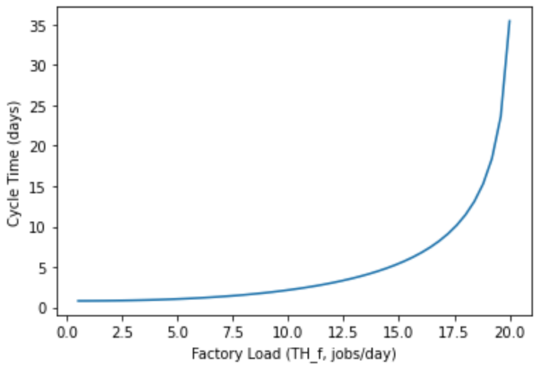
显然, 随着 factory load 的上升, cycle time 呈现指数级的增长. 那么有什么办法可以缓解这种爆炸增长呢?

减少 variability
增加瓶颈 workstation 的 EPR_ws (capacity)

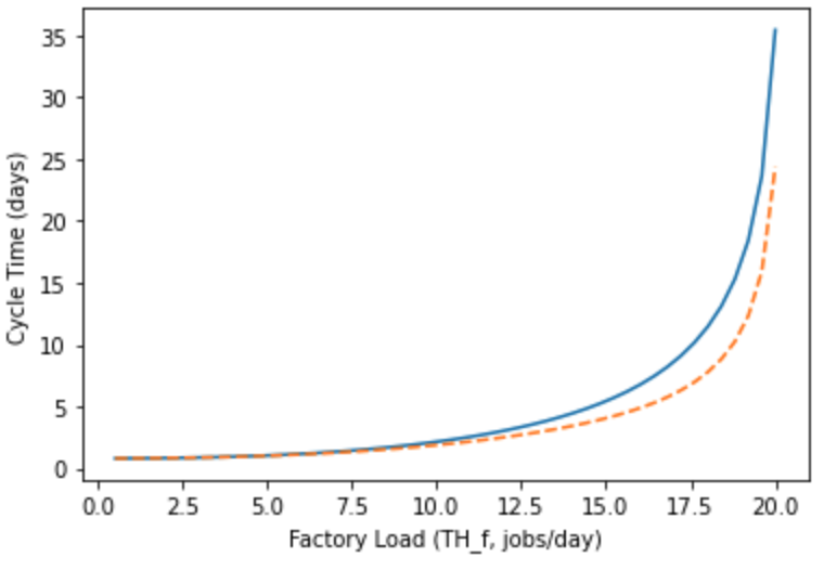
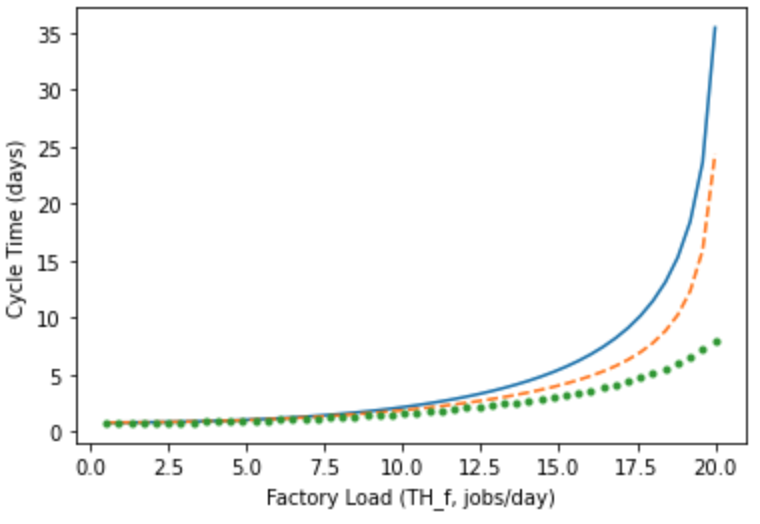
例如, (1) 在把 ws_A 的 cov_EPT 从 8 降低至 1 后:

(2) Based on (1) 在进一步把 ws_D 的 EPR_m 从 4.1 增加至 5 后:</u>

7.2 Load-Adjusted Cycle-Time Efficiency

Define Cycle-Time Efficiency (CTE) as the ratio of the process time to the cycle time:

C T E_{f} = \frac{{Process Time}_{f}}{C T_{f}}

We define a factory’s process time as that which includes the time devoted to all value-added as well as non-value-added process steps. Alternative representations of factory cycle-time efficiency omit any non-value-added process step time (e.g., time consumed by transit, inspection, or test).

但是, 我们无法将现在的 $C T E$ 作为一个工厂的评价标准: 如下表, 不难发现 Loading 越低 CTE 就越大, 这是毫无意义的

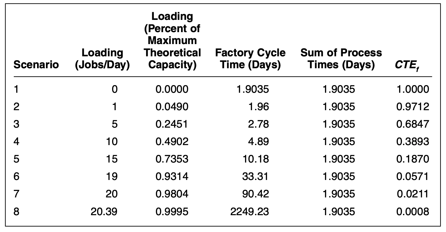
因此为了使 $C T E -$ metric 有意义, we have to make it adjustable to factory loading. 因此定义 load-adjusted cycle-time efficiency (LACTE) 为:

L A C T E_{loading} = \frac{{Process Time}_{f}}{C T_{f}} \times \frac{T H_{f}}{T H_{f}^{*}}

$T H_{f}^{*}$ : maximum theoretical factory capacity
$T H_{f}$ : actual factory throughput

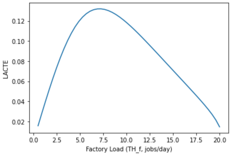
例如, 还是对于 Section 7.1 中的 nonreentrant 5-workstations factory, 我们可以画出 plot of LACTE vs. factory load:

代码实现: FabSim_1_7.py

LACTEs = []
TH_f_max = 0
for TH_f in np.linspace(0.5, 20, 50):
    ws_A = WorkStation(TH_f=TH_f, cov_AR=8, cov_EPT=8, m=6, EPR_m=4)
    ws_B = WorkStation(TH_f=TH_f, cov_AR=ws_A.cov_DR, cov_EPT=2, m=3, EPR_m=10)
    ws_C = WorkStation(TH_f=TH_f, cov_AR=ws_B.cov_DR, cov_EPT=3, m=4, EPR_m=8)
    ws_D = WorkStation(TH_f=TH_f, cov_AR=ws_C.cov_DR, cov_EPT=3, m=5, EPR_m=4.1)
    ws_E = WorkStation(TH_f=TH_f, cov_AR=ws_D.cov_DR, cov_EPT=2, m=3, EPR_m=9.5)

    f = Factory(TH_f=TH_f)
    f.add_workstations([ws_A, ws_B, ws_C, ws_D, ws_E])
    LACTEs.append(f.calLACET())
    TH_f_max = f.TH_f_max

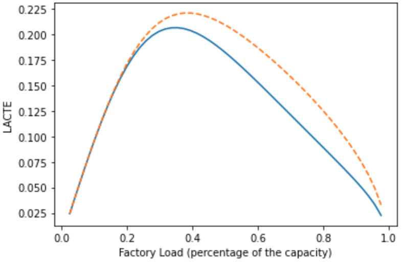
plt.xlabel("Factory Load (percentage of the capacity)")
plt.ylabel("LACTE")
plt.plot(np.linspace(0.5, 20, 50)/TH_f_max, LACTEs)

类似 Section 7.1, 降低 variability 后的工厂有更好的表现

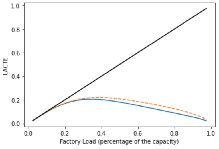
LACTE Evnvelope

如下图黑线, 这里的 envelope 可以理解为 factory performace 的上界, 即一种 utopian (乌托邦式的) 理想状态: 该状态下 variability = 0

7.3 Profit Curve

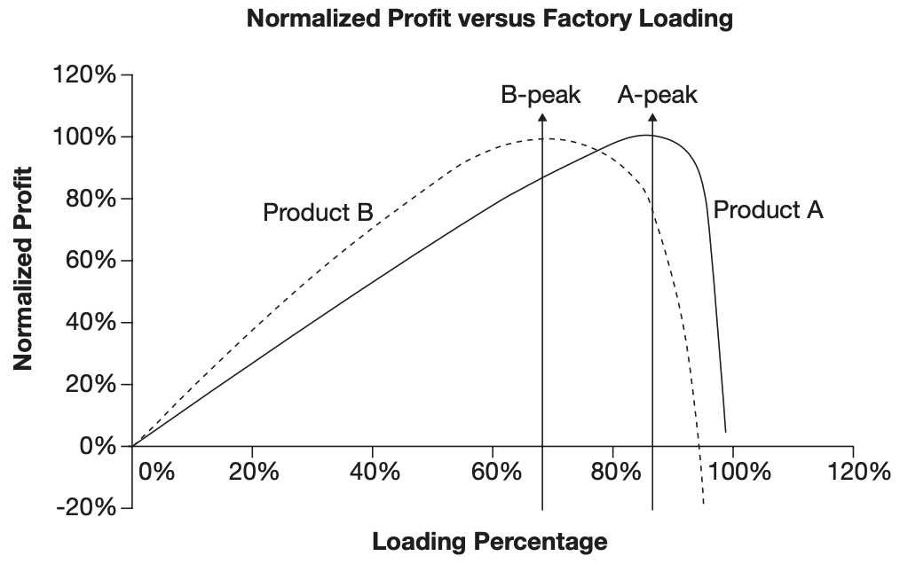
The factory profit curve serves to estimate that optimal level of loading. Derivation of the profit curve requires, as a first step, the development of estimates of profit over a given planning horizon

例如现有以下两种产品 Product A, Product B, 分别由 Factory A, Factory B 生产 (这两个工厂除了生产不同的产品外, 其他参数都一样)

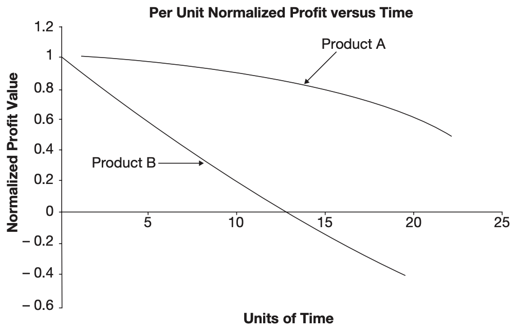
Figure: Profit versus time plots, products A and B

由于两个产品不同的 profit vs. time plot, 两个工厂的 profit curve 也不同:

Figure: Factory profit curves for factories A and B

8. Factory Performance Metrics: The Good, the Bad, and the Ugly

Good Metrics:

Waddington effect plot
M-ra

30-period

work with model team

sounds good

有一个线上的liscense type（但是目前只用）

和gurobi合作，make presentation时叫上他们

service

Document Information

Author: Zeka Lee
Link: https://zhekaili.github.io/0007/10/01/Book-Optimizing-Factory-Performance/
Copyright: 自由转载-非商用-非衍生-保持署名（创意共享3.0许可证）

Book - Optimizing Factory Performance