加工时间 takt time = 1/throughput rate

6. A Science of Manufacturing

6.1 The Seeds of Science

6.1.1 Why Science?

Example: Factory Design

Suppose the VP of manufacturing has demanded that a printed-circuit board (PCB) plant produce

• 3,000 PCBs per week to meet demand.
• An average cycle time (delay between job release and completion) <= 1 week.
• No overtime (workweek of 40 hours), to keep costs low.

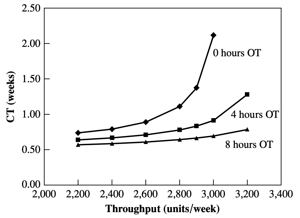
Can it be done? To answer this question, we must first generate the relationships(between cycle time and demand) for the PCB plant.

• $x-$axis indicates the throughput rate
• $y-$axis shows the resulting average cycle time
• The three curves show the relationship for the cases of no overtime, 4 and 8 hours of overtime per week

The curve show that if we insist on no more than 1 week for the average cycle time with no overtime, the best we can do is 2,600 units per week. If we insist on an average cycle time of less than 1 week and 3,000 units per week, we will need an additional 4 hours per week of overtime.

6.2 Formal Roots

6.2.1 “Formal Cause” of Manufacturing Systems

7. Basic Factory Dynamics

7.3 Simple Relationships

7.3.1 Best-Case Performance

Law (Little’s Law):

where $\text{WIP}$ (work in process), $\text{TH}$ (throughput), $\text{CT}$ (cycle time)

Law (Best-Case Performance):

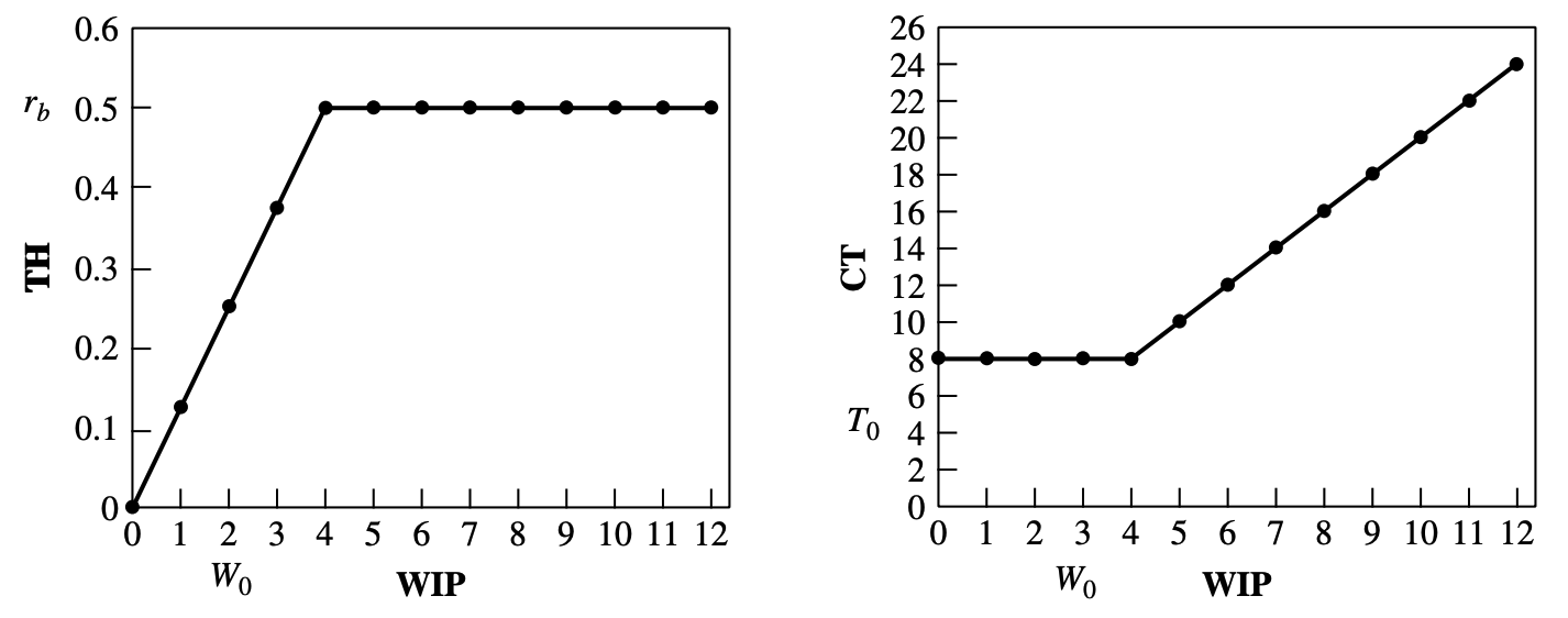
The minimum cycle time for a give WIP level $w$ is given by:

The maximum throughput for a given WIP level $w$ is given by:

where

• $T_0$ min cycle time
• $r_b$ max throughput
• $W_0=T_0r_b$ a critial WIP

7.3.2 Worst-Case Performance

7.3.3

需要继续看

8. Variability

8.1 - 8.2

没有什么实质内容，略

8.3 Process Time Variability

cov (CV): If we let $t$ denote the mean (we use t because the primary random variables we are considering here are times) and $\sigma$ denote the std:

sqared cov (SCV):

8.4 Causes of Variability

The most prevalent sources of variability in manufacturing environments are:

• “Natural” variability, which includes minor fluctuations in process time due to differences in operators, machines, and material.
• Random outages.
• Setups.
• Operator availability.
• Rework

8.4.1 Natural Variability

Natural variability is the variability inherent in natural process time, which excludes random downtimes, setups, or any other external influences.

In most systems, natural process times are LV (low variability) and so $c_0 < 0.75$

8.4.2 Variability from Preemptive Outages (Breakdowns)

8.5 Flow Variability

All the above discussion focused solely on process time variability at individual workstations. But variability at one station can affect the behavior of other stations in a line by means of another type of variability, which we call flow variability

8.5.1 Characterizing Variability in Flows

Characterize Arrivals. Define:

• $t_a$: mean time between arrivals to a workstation
• $r_a$: arrival rate (jobs per unit time)

Set $t_e, r_e$ (mean process time, throughput) to describe the capacity of a workstation, in order for the workstation to be able to keep up with arrivals, it is essential that capacity exceed the arrival rate:

Arriveal time is also varaible, arrvial CV (defer to process time CV $c_e$)

Low CV Arrivals vs. High CV Arrivals

Characterize Departures. Define:

• $t_d$: mean time between departures from a workstation
• $r_d$: departure rate $=1/t_d$
• $c_d$: departure CV

In a serial line, the departure rate is the same as the arrival rate at the next station:

same for CV:

Utilization $u$. Assume there’are $m$ identital machines in a workstation:

Note that the max utilization is $1$, which means:

Relate $c_a$ and $c_d$: (1) One machine at a station $m=1$

• when $u\to 1$, the station is always busy, so the CV of interdepartures (描述两个连续离开 station 的物体之间的时间间隔) is dominated by the CV of process times $c_d=c_e$
• when $u\to 0$, the station is very lightly loaded, so the CV of interdepartures is dominated by the CV of arrivals $c_d=c_a$

(2) Multiple machines at a station $m>1$

8.5.2 Demand Variability and Flow Variability

?

8.5.3 Batch Arrivals and Departures

One important cause of flow variability is batch arrivals.

?

8.6 Variability Interactions—Queueing

A queueing system combines:

• an arrival process: Arrivals can consist of individual jobs or batches. Jobs can be identical or have different characteristics. Interarrival times can be constant or random.
• a service (i.e., production) process: The workstation can have a single machine or several machines in parallel, which can have constant or random process times.
• a queue: The queueing discipline can be first-come, first-served (FCFS); last-come, first-served (LCFS); earliest due date (EDD); shortest process time (SPT); or any of a host of priority schemes. The queue space can be unlimited or finite. The variety of queueing systems is almost endless

8.6.1 Queueing Notation and Measures

Assume we know:

• $r_a=$ arrival rate (jobs per unit time) to station. In a serial line without yield loss or rework, $r_a=\text{TH}$ (throughput)
• $t_a=1/r_a$: mean time between arrivals
• $c_a=$ arrival CV
• $m=$ number of parallel machines at station
• $b=$ buffer size (maximum number of jobs allowed in system)
• $t_e=$ mean effective process time
• $r_e=m/t_e$ the capacity (rate) of the workstation
• $c_e=$ effective process time CV

Performace measures we will focus on:

• $p_n=$ probability that there are $n$ jobs at station
• $\text{CT}_q=$ expected waiting time in queue
• $\text{CT}=$ expected time spent at system (queue time + process time)
• $\text{WIP}_q=$ expected number of jobs in queue
• $\text{WIP}=$ expected number of jobs at system (queue + workstation)

Kendall’s notation for queueing systems:

where $A$ describes the distribution of interarrival times, $B$ describes the distribution of process times, $m$ is the number of machines at the station, and $b$ is the maximum number of jobs that can be in the system. Typical values for $A$ and $B$, along with their interpretations, are

• $D$: constant (deterministic) distribution
• $M$: exponential (Markovian) distribution
• $G$: completely general distribution (e.g., normal, uniform)

In many situations, queue size is not explicitly restricted (e.g., the buffer is very large). We indicate this case as $A/B/m/∞$ or simply as $A/B/m$.

8.6.2 Fundemental Relations

Utilization $u$:

Others:

8.6.3 $M/M/1$ Queue

This model assumes exponential interarrival times, a single machine with exponential process times, a FCFS protocol, and unlimited space for jobs waiting in queue.

Because the interarrival and process time distributions are memoryless (exponantial distribution), the time since the last arrival and the time the current job has been in process are irrelevant to the future behavior of the system.

Because of this, the state of the system can be expressed as a single number $n$, representing the number of jobs currently in the system. And also because of the exponential distributions, we only need to know $t_a,t_e$ (so that $r_a, r_e$)

Define:

• $p_n=$ long-run probability of finding the system in state $n$ ($n$ jobs at workstation)
• For a system in state $n$, it can only transfer to state $n+1$ (a job arrives) or state $n-1$ (a job departs)
  • $p_{n-1}r_a=$ unconditional rate at which the system moves from state $n-1\to n$
  • $p_nr_e=$ rate to move from state $n\to n-1$

In order for the system to be stable, these two rates must be equal:

Since the machine is idle only when there are no jobs in system (系统空闲的概率 = 1 - utlization):

$\text{WIP}$ expected number in system (queue + workstation)

$\text{CT}$ average time in system. Since $\text{WIP} = \text{TH} \times \text{CT}$, and here $\text{TH} = r_a = ur_e = u/t_e$, we have:

$\text{CT}_q$ average time in queue

$\text{WIP}_q$ expected number in queue

8.6.5 $G/G/1$ Queue

The approximation for $\text{CT}_q$ , which was first investigated by Kingman (1961) (see Medhi 1991 for a derivation), is given by

• $V=$ variability term
• $U=$ utilization term
• $T=$ time term

8.6.6 $M/M/m$ Queue

8.6.7 $G/G/m$ Queue