2. Planning & Procurement

2.3 Demand Forecasting

• Qualitative Methods: when little historical data to rely on, intuition or expert judgement is required
• Quantitative Methods: when historical data exists and is helpful in calculating future demand

2.3.1 Quantitative Forecasting Methods

• Time Series: models that predict future demand based on past history
• Causal Relationships: models that use statistical techniques to establish relationships between demand various outside factors
• Simulation: models that can incorporate some randomness and non-linear effects

2.3.2 Type of Demand Patterns

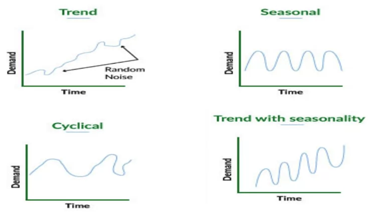
2.3.3 Time Series: Moving Average

\(F_{t+1}=\frac{A_t+A_{t-1}+...+A_{t-n}}{n}\)

where, $F_{t+1}$ is the forecast for next period $A$ is the actual sales figure from each period

2.4 Replenishment Planning

2.4.1 Independent and Dependent Demand

• Independent Demand: Customer demand for a finished product
• Dependent Demand: The demand for required component parts or subassemblies

2.4.2 Reorder Points

Fixed Order Quantity:

• Same amount of prodcut is ordered
• Order placement time varies
• When on hand inventory reaches pre-determined reorder point (ROP), the standard quantity is ordered
• ROP quantity is the amount of inventory needed to cover demand over then replenishment lead time

Fixed Order Interval:

• Product order amount varies
• Order time interval remains constant
• The inventory level is observed when the reorder time comes. Replenish order is placed to allow to inventory reach the desired level

2.4.3 Economic Order Quantities

Assumptions:

• Constant annual demand $D$
• Replenishment lots are always received in full requested quantities

Notations:

• $Q$: order quantity
• $C$: cost per unit
• $h$: holding cost
• $S$: cost per order

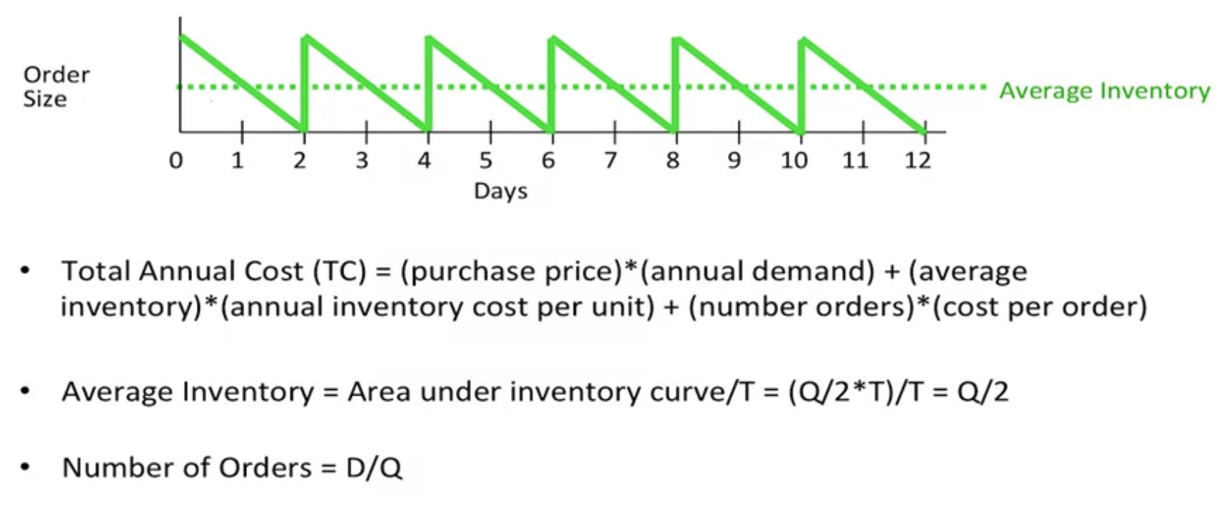
take $dC_T/dQ=0$, we have Optimal Order Quantity \(Q^*=\sqrt{\frac{2DS}{hC}}\)

Others

Stock Coverage (Inventory Coverage): \(\text{Stock Coverage (days)}=\text{Net Stock/ Avg. daily unit sales}\)

Capacity: Capacity is always m / processing time with m being the number of resources (e.g. workers) being devoted to the station. If, for example, one worker needs 40 seconds to put together a sandwich, the capacity of this station is 1.5 sandwiches per minute. If there are two workers on the same station, the capacity increases to 3 sandwiches per minute.

Bottleneck: The bottleneck is defined as the process step (station) in the flow diagram with the lowest capacity (the “weakest link”). (although the bottleneck is often the process step with the longest processing time)

Process Capacity: The process capacity is always equivalent to the capacity of the bottleneck.

Flow rate: \(\text{Flow Rate}=\min\{\text{Demand, Process Capacity}\}\)

Utilization: The utilization tells us, how well a resource is being used. It is calculated as flow rate divided by capacity (e.g. 1/25). The utilization always lies between 0% and 100%.

Guest Lec