Two types of inventory polices: continuous view vs. periodic view

Three performance measures: $E[Cost]$ and two service measures (stockout probability and fillrate

1. EOQ with Uncertain Demand (Ch 16.6)

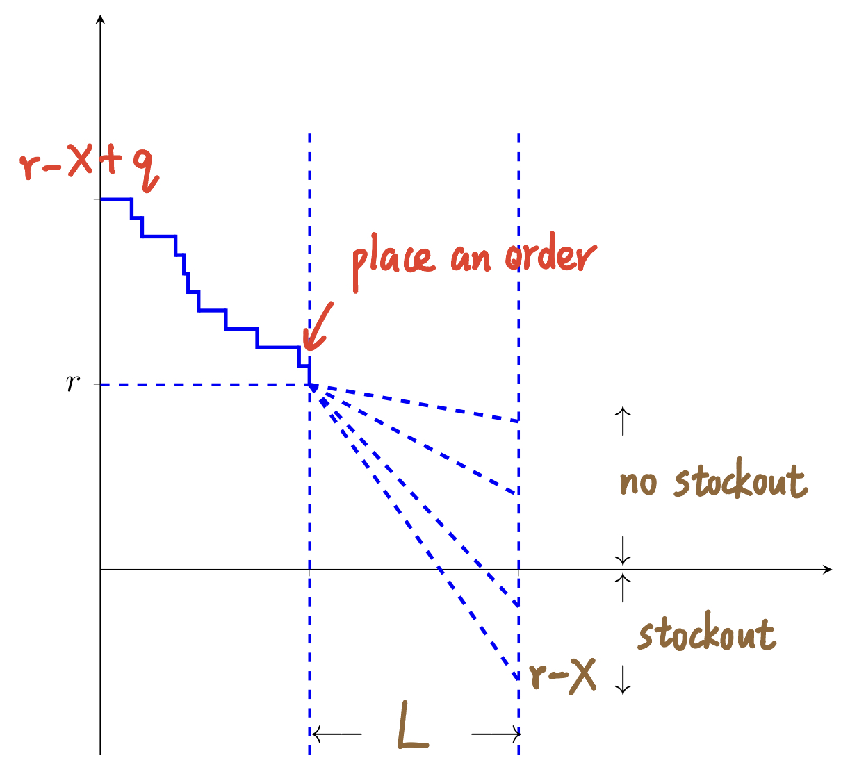
The EOQ model is a continuous review poliy (inventory level can be monitored continuously in time and an order is placed as soon as the inventory level hits a reorder point)

• $K=$ set up cost per order
• $h=$ holding cost per item per time
• $L=$ lead time (positive, could be constant or stochastic)
• $D=$ demand (annually, stochastic)
• $c_B=$ backorder cost per item
• $OHI(t)=$ on-hand (on hand) inventory at time $t$
• $B(t)=$ # backordered items at time $t$
• $I(t)=OHI(t)-B(t)$
• $B_r=$ # backordered items during the lead time with reorder point $r$
• $q=$ order quantity

  (decision varaible)

• $r=$ reorder point

  (decision varaible)

Derived Notations:

• $ss = r-E[X]$ (safety stock)
• average stock level $=ss+q/2$

$X$ is a random variable representing demand during lead time

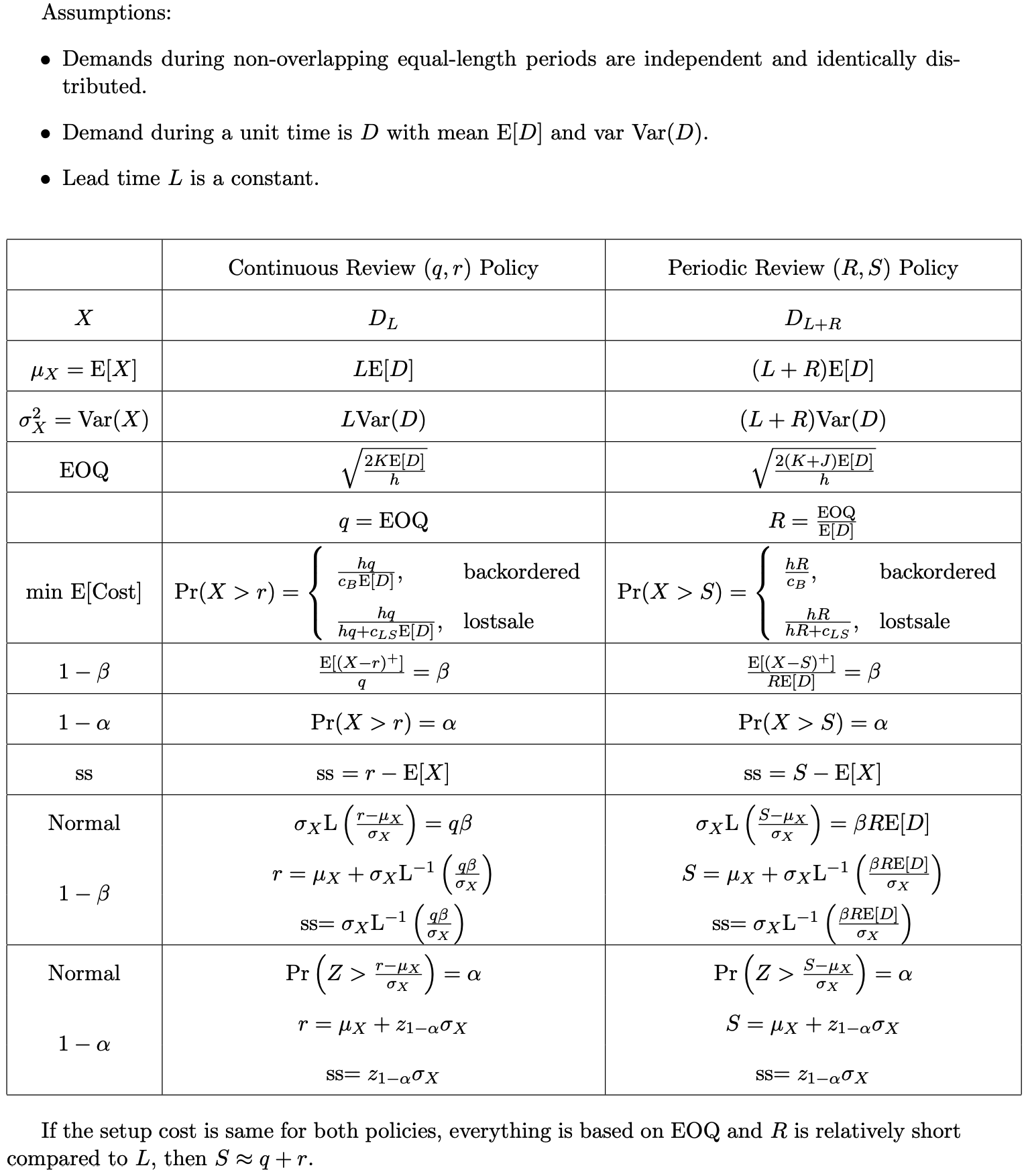
• If demand during each period is independent and $L$ constant \(E[X]=L\cdot E[D]\text{ and }Var(X)=L\cdot Var(D)\)
• If demand during each period is independent, as well as $L$ \(E[X]=E[L]E[D]\text{ and }Var(X)=E[L]Var(D)+E^2[D]Var(L)\)

1.1 Back-ordered Case

Back-ordered means that the customer still want the late items, but we need to pay some compensate (back-ordered cost). Equation of total cost: \(TC(q,r)=\text{set up cost + holding cost + backordered cost + no-care}\)

• ”$\text{no-care}$” indicates the costs that have nothing to do with $q,r$, including purchasing cost ($E[D]p$), in-transit cost ($E[D]Lh$)

\[\begin{aligned} TC(q,r) &=K\frac{E[D]}{q}+h\cdot\frac{1}{2}[(r-E[X]+q)+(r-E[X])]+c_BE[B_r]\frac{E[D]}{q} \\ &=K\frac{E[D]}{q}+h(r-E[X]+\frac{q}{2})+c_BE[B_r]\frac{E[D]}{q} \\ \end{aligned}\]

To find the optimal $q$ and $r$, we need the expression of $E[B_r]$ and $\frac{\partial}{\partial r}E[B_r]$:

• $E[B_r]=E[(X-r)^+]=\int_r^\infty(x-r)f(x)dx$
• $\frac{\partial}{\partial r}E[B_r]=-\text{Pr}(X>r)$

关于公式 $\frac{\partial}{\partial r}E[B_r]$ 的理解: 该公式的数值随着 $r$ 的增加逐渐从 $-1\to 0$, 这意味着 $E[B_r]$ 将是一个单调递减的函数，符合我们的直觉(reorder point 越大, stockout 的数量越少)

Special Case: normally distributed $X$ (a) Firsly definde the normal loss function $L(\cdot)$ \(L(c)=E[(Z-c)^+]=\phi(c)-c(1-\Phi(c))\)

where $Z\sim N(0,1)$; $\phi,\Phi$ are standard pdf and cdf (b) Lemma: \(L(-c)=c+L(c)\)

(c) Then for $X\sim N(\mu_X,\sigma^2_X)$ \(E[B_r]=E[(X-r)^+]=\sigma_XL(\frac{r-\mu_X}{\sigma_X})\)

(d) Finally we are ready to calculate the optimal $q$ and $r$ (导数为 0): \(q^*=\sqrt{\frac{2E[D](K+c_BE[B_r])}{h}}\text{ and Pr}(X>r^*)=\frac{hq^*}{c_BE[D]}\)

Note: there is a bug that $q^*,r^*$ are dependent to each other. Two approaches:

• Heuristic (启发式的): approximate $q^$ by $\text{EOQ}=\sqrt{2KE[D]/h}$, then solve $r^$
• Exact: start with EOQ and solve iteratively until $(q,r)$ converges

Remarks:

1. $q^*\geq EOQ$ due to extra $c_BE[B_r]$ term
2. $r^*\geq E[X]$ due to $c_B\geq p$ and uncertainty in $X$
3. As $r\uparrow$, inventory $\uparrow$, $E[B_r]\downarrow$, $q\downarrow$
4. As $q\uparrow$, total holding cost $\uparrow$, total set up cost $\downarrow$, and $r\downarrow$ (total shortage cost $\uparrow$)
5. As $h\uparrow$, both $q^,r^\downarrow$

1.2 Lost Sales Case

Lost Sales means customer **will not want any late items**, therefore cost of lost sales per item per time is: \(c_{LS}=c_B+\text{(sale price - sell price)}\)

\[TC(q,r)= K\frac{E[D]}{q}+h(r-E[X]+E[B_r]+\frac{q}{2})+c_{LS}E[B_r]\frac{E[D]}{q}\] \[q^*=\sqrt{\frac{2E[D](K+c_{LS}E[B_r])}{h}}\text{ and }Pr(X>r^*)=\frac{hq^*}{hq^*+c_{LS}E[D]}\]

2. Service Levels for a Continuous-Review Policy (Ch 16.7)

The problem of using total cost to find $q^,r^$ is that it’s hard to quantify the values of $c_B,c_{LS}$ (up to the customers).

2.1 Fillrate

$\text{Fillrate}=1-\beta$: the expected fraction of demand met on time

Special Case: normally distributed $X$ From the last part of section 1.1, we have \(\beta = \frac{\sigma_XL(\frac{r-\mu_X}{\sigma_X})}{q}\)

2.2 Stockout Probablity

$\text{Stockout Probablity}=\alpha=\text{Pr}(X>r)$

• Expected number of cycles with stockout for a year = $\alpha(E[D]/q)$

Quick Approach:

1. set $q^*=EOQ$
2. solve $r$ for either $\alpha$ or $\beta$

Useful properties of Gamma (a) If $G_1,G_2\sim\Gamma(k,\theta)$ and they are independent, then $G_1+G_2\sim\Gamma(k_1+k_2,\theta)$ (b) If $G\sim\Gamma(k,\theta)$, then $cG\sim\Gamma(k,c\theta)$ for a real constant c

3. Order Up To Policy // Base-stock Policy (Ch 16.8)

This is a periodic review policy: Every $R$ periods, we order up to $S$. When we implement it, we observe the on-order inventory, and place a replenishment order every R period in the amount of

• $D=$ annual demand
• $K=$ setup cost per order
• $J=$ cost of reviewing inventory level
• $h=$ holding cost per item per year
• $c_B=$ backordered cost per item
• $L=$ lead time
• $D_R=$ demand during $R$
• $D_{L+R}=$ demand during $L + R$ time
• $B_S=$ # demand not met on time during a cycle

Our decision variables are order-up-to quantity $S$ and review period $R$

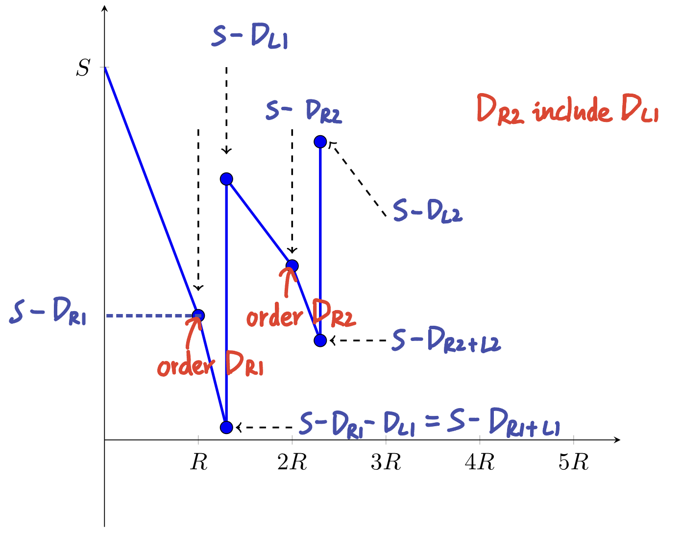
where

1. Orders are placed at $R,2R,3R,…$
2. Cycle periods are $[nR+L,(n+1)R+L],n=1,2,…$
3. Inventory level at each:
   • Cycle start point $=S-D_L$ (In picture above, the first cycle start at $S-D_{L1}$)
   • Cycle end point $=S-D_{R+L}$
   • Review period $=S-D_R$
4. Expected order quantity $=E[D_R]=RE[D]$
5. Stockout occurs when $S-D_{R+L}<0\iff S-D_R\leq D_L$
6. The expected number of lost demand is: \(E[B_S]=E[(D_{L+R}-S)^+]\)

3.1 Minimize Expected Total Cost

Backordered Case: By solving $\partial E[TC(R,S)]/\partial S$

\[\text{Pr}(D_{L+R}>S)=\frac{hR}{c_B}\]

In $(q,r)$, when we replace $q$ by $q\approx E[D_R]=RE[D]$, we have \(\text{Pr}(X>r)=\frac{hq}{c_BE[D]}\approx\frac{hR}{c_B}\)

Lostsale Case:

\[\text{Pr}(D_{L+R}>S)=\frac{hR}{hR+c_{LS}}\]

Similarly, in $(q,r)$ \(\text{Pr}(X>r)=\frac{hq}{hq+c_{LS}E[D]}\approx\frac{hR}{hR+c_{LS}}\)

Determination of $R$: If a company uses the $(R,S)$ policy, it is likely that $R$ is given. But if it’s not given and has to be determined, then one may want to make the shape of $I(t)$ graph resembling EOQ graph \(\text{number of orders}=\frac{E[D]}{EOQ}=\frac{1}{R}\)

then

\[R=\frac{EOQ}{E[D]}\text{ and }EOQ=\sqrt{\frac{2(K+J)E[D]}{h}}\]

3.2 Service Measures

Fillrate:

\[\text{Unfillrate}=\beta=\frac{E[B_S]\frac{1}{R}}{E[D]}\]

where $E[B_S]=E[(X-S)^+]=E[(D_{L+R}-S)^+]$

For normally distributed demand: ||constant $L$| r.v. $L$| |-|-|-| |$X=$|$D_{L+R}$| $D_{L+R}$| |$\mu_X=$| $(L+R)E[D]$| $E[L+R]E[D]=(E[L]+R)E[D]$ |$\sigma^2_X=$| $(L+R)\sigma^2_D$| $E[L+R]\sigma_D^2+Var(L+R)E^2[D]$| |$E[B_S]=$| $\sigma_XL(\frac{S-\mu_X}{\sigma_X})$|

Stockout:

\[\alpha=\text{Pr(Stockout)}=\text{Pr}(X>S)=\text{Pr}(D_{L+R}>S)\]

For normally distributed demand, \(\text{Pr(Stockout)}=1-\Phi(\frac{S-\mu_X}{\sigma_X})\)

4. $(s,S)$ Policy

Useful when orders come in bulk.

Continuous $(s, S)$:

• As soon as the $OOI(t)<s$ (on-order inventory at time $t$), order $S-OOI(t)$
• Very difficult to find the optimal $s$ and $S$. Using the fact that it is similar to the $(q, r)$ policy, one can approximate: \(s = r\text{ and }S = q+r\)

Periodic $(s, S)$:

• Inventory is checked only every fixed interval. Let $n$ represent the end of each review interval.
• If $OOI(n)\leq S$, order $S-OOI(n)$
• Otherwise, do not order
• Difficult to find the optimal $s$ and $S$. For a simple model, a discrete-time Markov chain can be used to find the optimal $s$ and $S$.